Este artículo presenta las matemáticas de la reconstrucción de luces de Ansel: el diseño original de 2021 de los
guided laplacians, cuyas ideas generales solo se habían esbozado en el foro pixls.us,1 y la transposición armónica,
el método que lo reemplazó tras un estudio con verdad de referencia (ground truth) que
expuso un fallo de recuperación de magnitud.2 Está organizado de modo que cada lector encuentre su
sección: los resultados y la sección Intuición y contexto de cada método no necesitan
matemáticas; los desarrolladores encontrarán las subsecciones de Implementación y optimizaciones y el
estudio de rendimiento; los
hallazgos teóricos y el
anexo del cementerio están escritos para ser
reutilizables fuera de la fotografía; y
cómo se hizo realmente este trabajo documenta el protocolo de
investigación hombre-máquina que hay detrás.
Resumen
Cuando el sensor de una cámara se satura, los tres canales de color no se recortan al mismo tiempo, de modo que una alta luz quemada deriva en color, normalmente hacia el magenta. Este artículo documenta la reconstrucción de luces de Ansel de principio a fin y en el orden en que sucedió: los guided laplacians originales de 2021 (transferencia de detalle de wavelet a través de un filtro guiado, nunca antes plasmada por completo), el estudio con verdad de referencia que expuso su fallo de magnitud, y el método que lo reemplazó: la transposición armónica, que conserva el modelo local de línea de color del filtro guiado pero transporta sus coeficientes a través de la zona quemada como campos suaves difundidos, guiados por la estructura de los canales supervivientes, corrige el sesgo del declive de saturación del sensor antes de ajustar, y entrega cada banda de frecuencia y clase de píxel al estimador que es medible como el mejor allí. Cada decisión de diseño está respaldada por un número en un banco de pruebas público, y los fracasos se documentan con el mismo cuidado que los éxitos, incluidos dos resultados que creemos generales: la energía de costura en cualquier traspaso entre estimadores es igual al desacuerdo entre los estimadores y no puede ponderarse para eliminarla, y la validez de una línea de color en lo profundo de una zona quemada es indecidible a partir de los datos que la rodean.34
El problema
El tinte magenta
Un sensor digital es una matriz de fotositos, cada uno cubierto por un filtro de color de una matriz de filtros de color (CFA): el patrón de Bayer (2×2 de R, G, G, B) o el X-Trans de Fuji (6×6). Cada fotosito es un pozo potencial que se llena de fotoelectrones durante la exposición y se satura a una capacidad fija. Como la capacidad del pozo es una propiedad del silicio, los tres colores se saturan aproximadamente al mismo valor de código raw.
La trampa es el balance de blancos. Un sujeto gris neutro no produce señales raw iguales en los tres canales: las transmisiones de la CFA, la sensibilidad espectral del sensor y el iluminante de la escena difieren todos por canal. Para representar tal sujeto como neutro, el revelador raw multiplica cada canal por un coeficiente de balance de blancos: normalmente el canal verde se deja cerca de $1$ mientras que el rojo y el azul se multiplican hasta $1.5$ o $2$.
Ahora sigue una alta luz neutra a medida que se vuelve más brillante. En el sensor no hay nada por canal en la saturación: las tres señales raw suben hacia un techo compartido —el pozo lleno— y se recortan a más o menos el mismo valor. El magenta se fabrica después, por las ganancias del balance de blancos: multiplicar cada canal cambia tanto su pendiente al subir como el nivel en el que aterriza su meseta recortada. El verde (ganancia $\approx 1$) forma meseta donde el sensor lo dejó; el azul y el rojo son empujados hacia arriba por sus ganancias y forman meseta por encima de él. Pasada la saturación las proporciones registradas ya no son neutras —el rojo y el azul sobrepasan al verde, y la alta luz “blanca” se lee como magenta. (En sujetos reales los canales sí se recortan en secuencia —el color propio del sujeto y las sensibilidades por canal escalonan los inicios, razón por la cual existen píxeles parcialmente recortados que portan guías supervivientes— pero el magenta de un neutro quemado es obra de las ganancias, no de umbrales por canal.)
Note
Este es un artefacto puramente mecánico y colorimétrico del aparato de captura. No hay magenta en la escena. Cualquier reconstrucción que trabaje en un espacio de color después del interpolación cromática ya está luchando contra un error de tono que un algoritmo de interpolación cromática habrá emborronado por los píxeles vecinos. Reconstruir antes del interpolación cromática, mientras los datos siguen siendo un mosaico limpio por canal, es la razón de ser del método guided-laplacian.
El valor en el que se declara recortado un canal no es el máximo numérico sino un umbral por canal derivado del punto blanco raw:
donde $\text{white}_c$ es el processed_maximum del módulo para el canal $c$ (el nivel de blanco raw
por canal que sobrevive a las etapas anteriores del pipeline) y clip es un factor de seguridad del usuario en torno a $1$.
El margen $0.995$ mantiene los fotositos casi saturados (cuya respuesta ya se ha vuelto no lineal
cerca de la cima del pozo) fuera del conjunto “válido”.2
Arreglos más simples
El módulo de Ansel ofrece tres modos de reconstrucción más baratos antes del de guided-laplacian, y vale la pena enunciarlos porque enmarcan lo que compra el método caro:
- Clip simplemente aplasta cada canal al umbral común $\texttt{clip}\times\min_c \text{white}_c$ (los mismos niveles de blanco, sin el margen $0.995$). Sin magenta, pero cada región recortada se convierte en un pegote blanco plano y sin textura.
- Reconstruir en LCh convierte cada bloque de Bayer en un triplete de luminancia/croma/tono, reescala el croma de los bloques recortados para que coincida con la luminancia no recortada, y vuelve a convertir. Elimina la deriva de tono pero no puede inventar textura.2
- Reconstruir color (inpaint) propaga proporciones de color desde los píxeles no recortados vecinos a lo largo de filas y columnas, usando la actualización de proporciones de decaimiento exponencial del algoritmo de Magic Lantern. Es rápido y direccional pero unidimensional y fácilmente engañado por bordes complejos.2
El modo guided laplacians es el único que restaura tanto la textura como la magnitud de
una región recortada, tomando prestado de los canales que sí sobrevivieron a lo largo de la línea de color local.
Darktable anterior incluye dos modos de reconstrucción que Ansel no lleva, y ofrecen una comparación instructiva porque parten de una suposición diferente sobre lo que es una alta luz quemada. Ambos fueron desarrollados por los equipos de G’mic y Darktable y ambos trabajan, como nuestro método, sobre el mosaico raw: cada canal de color se aproxima primero en todas partes a partir de su vecindario de fotositos 3×3, dando una imagen por canal tosca pero de resolución completa.
Inpaint opposed descansa sobre una observación empírica: para un canal recortado, la media de los otros dos canales (la media “opuesta”, calculada en el espacio de raíz cúbica para comprimir el rango dinámico) es una buena estimación del valor perdido en la inmensa mayoría de las imágenes. El mecanismo es en consecuencia simple: reemplazar cada valor recortado por esa media opuesta, luego añadir un desplazamiento de crominancia global, medido sobre los píxeles morfológicamente más cercanos a las zonas recortadas, para absorber el tinte de color general. Sus modos de fallo documentados son las escenas donde una relación fija no puede sostenerse: iluminación mixta, balance de blancos lejos de la suposición del pipeline, o varias fuentes de luz con colores diferentes alimentando distintas luces.
Segmentation based refina el mismo estimador base con adaptación espacial. Los píxeles recortados de cada canal se rellenan por inundación en segmentos conexos (opcionalmente fusionados por un cierre morfológico, el control “combine”); para cada segmento, el algoritmo busca en su borde no recortado el mejor píxel candidato (puntuado por la desviación estándar local y la mediana en una ventana 5×5) y trasplanta la pseudocrominancia de ese candidato (el canal menos la media opuesta, de nuevo en el espacio de raíz cúbica) por todo el segmento. Si no existe un candidato convincente, recurre a una media de segmento completo con una corrección de crominancia. Donde todos los canales se recortan, una pasada de “rebuild” separada extrapola una superficie de luminancia a partir de los gradientes del borde, controlada por una transformada de distancia —el pariente más cercano, en todo este panorama, de nuestra cúpula biarmónica. Las suposiciones son, pues: una crominancia representativa por segmento (mejor que una por imagen, pero aún plana dentro de un segmento), textura heredada de lo que porten los canales supervivientes, y extrapolación de gradiente donde nada sobrevivió.
Ambos son intentos desesperados de rellenar el área dañada con algo plausible, pero promueven superficies coloreadas planas a la magnitud equivocada.
Primeros principios
El método es un ensamblaje de cuatro ideas. Dos de ellas (los laplacianos discretos y la pirámide B-spline à-trous) se comparten palabra por palabra con diffuse or sharpen y aquí solo se resumen. Las otras dos, el filtro guiado y la difusión de crominancia, cargan con la reconstrucción y se derivan por completo.
Gradientes y laplacianos
Para una imagen discreta $u(i,j)$, el gradiente mide la pendiente local,
y el laplaciano mide la curvatura local: cuánto se aparta un píxel de la media de sus vecinos,
El laplaciano es aquí el caballo de batalla porque aísla la textura como oscilación en torno a una media local (es cero en las regiones planas y solo responde al contraste local) y porque es lineal: sobreexponer o subexponer la imagen simplemente lo reescala (una propiedad en la que nos apoyamos abajo). Aislar la textura de esta manera es lo que nos permite trasplantarla entre canales sin arrastrar el brillo absoluto de la guía; la diferencia de magnitud global entre un canal recortado y su guía es absorbida por la pendiente del filtro guiado, no por el laplaciano en sí. Ansel usa la plantilla de 9 puntos rotacionalmente simétrica de Oono & Puri
cuyo error angular es mucho menor que el de la ingenua cruz de 5 puntos, de modo que la difusión no privilegia los ejes de la rejilla de píxeles.567
La pirámide de B-spline à-trous
Para actuar sobre estructuras de muchos tamaños, la imagen se divide en bandas de frecuencia difuminándola repetidamente con el núcleo B-spline cardinal separable
una aproximación compacta de una gaussiana de parámetro $\sigma_B \approx 1.0554$.8 En la escala $s$ los taps se separan con un paso de $2^s$ píxeles (“à-trous” = “con agujeros”), de modo que el mismo núcleo diminuto alcanza cada vez más lejos sin crecer nunca en coste. Escribiendo $G_s$ para las sucesivas imágenes paso-bajo (progresivamente difuminadas) y $H_s$ para las bandas de detalle,
la imagen es exactamente la suma de sus bandas, $u = \sum_{s=0}^{n-1} H_s + G_{n-1}$. Una banda de detalle $H_s$ es una diferencia de gaussianas, que es a su vez una aproximación escalada de un laplaciano-de-gaussiana —de modo que “filtrar la banda $H_s$” y “aplicar un laplaciano a la escala $s$” son dos vistas de la misma operación. La derivación completa, incluyendo cómo crece el radio gaussiano equivalente como
se da en el artículo complementario sobre diffuse or sharpen.29
Note
Abajo se usan dos productos de esta pirámide. El paso-bajo $G_s$ es una media local ponderada a la escala $s$ —exactamente la media local que el filtro guiado necesita, en toda una escalera de tamaños de ventana. La banda de detalle $H_s$ es un laplaciano escalado, el operador que integra el respaldo de difusión de crominancia. La reconstrucción propiamente dicha trabaja sobre los $G_s$ (que portan la magnitud del color); el respaldo trabaja sobre los $H_s$.
El filtro guiado
El filtro guiado de He, Sun y Tang es el motor que toma prestada textura de un buen canal hacia uno recortado.3 Supongamos que queremos producir una imagen de salida $q$ que se mantenga fiel a algún objetivo $p$ pero que lleve los bordes y la textura de una guía $I$. Supongamos que, dentro de cualquier ventana pequeña $\omega_k$ alrededor del píxel $k$, la salida es una función afín de la guía:
Esta única suposición, una línea de color local, es todo el modelo. Dice que dentro de un pequeño parche el canal que estamos reconstruyendo es solo una copia escalada y desplazada de la guía. Es el mismo prior que subyace al interpolación cromática entre canales, la eliminación de neblina, el matting de imágenes y la colorización: las superficies naturales trazan líneas de color (localmente, sus canales están relacionados de forma afín) porque la mayoría de los bordes son cambios en la reflectancia que escalan todos los canales juntos.10 Bajo un mapa afín, $\nabla q = a_k \nabla I$, de modo que $q$ hereda cada borde de $I$, meramente reescalado por $a_k$.
Ajustamos $(a_k, b_k)$ por mínimos cuadrados, manteniendo $a_k$ pequeño para evitar amplificar el ruido (un término de cresta $\varepsilon a_k^2$):
Igualar las derivadas a cero da la forma cerrada que aparece, casi palabra por palabra, en el código:
La covarianza en el numerador (una medida de cuánto suben y bajan juntos la guía y el objetivo) es la clave: donde se mueven juntos, $a_k \to 1$ y la textura de la guía se copia; donde la guía es plana ($\operatorname{var} \to 0$), $a_k \to 0$ y la salida recurre a la media local $\bar p$. El parámetro de cresta $\varepsilon$ fija la escala por debajo de la cual las variaciones se tratan como ruido y se suavizan en lugar de transferirse.
Note
El filtro guiado de He tiene un segundo paso (promediar los coeficientes por ventana $(a_k, b_k)$ sobre todas las ventanas que cubren un píxel) que evita que la salida se vea a bloques. La implementación reconstruida obtiene el mismo suavizado gratis calculando la estadística de ventana con un núcleo suave (una gaussiana) en lugar de una caja dura: ventanas suaves solapadas hacen de $a$ y $b$ campos que varían suavemente, de modo que $a,I + b$ ya está libre de artefactos sin una pasada de promediado aparte. Esto no es un detalle cosmético: repetir el mismo ajuste con una ventana de caja dura de soporte comparable deja rayas visibles alineadas con los ejes y mesetas escalonadas dondequiera que la estructura de la imagen cruce el límite de una ventana, y cuesta cerca de un tercio más de error en la escena de bordes del banco de pruebas. El código de 2021, por su parte, usaba una caja dura $3\times3$ sin ningún promediado en absoluto —se salió con la suya porque la ventana tiene tres píxeles de ancho y la difusión iterada suaviza lo que deje detrás.[^impl]
La difusión como inpainting de color
Rellenar el color de un agujero es un problema diferente de rellenar su textura. El color de un agujero debería variar suavemente y coincidir con su borde; no debería portar detalle de alta frecuencia (textura fina y de variación rápida) propio. El formalismo natural es la energía de Dirichlet, la cantidad total de variación que contiene la imagen, grande donde se ondula y cero donde es constante:
cuyo minimizador sobre el agujero $\Omega$, con los píxeles circundantes como condición de contorno, es la función armónica que satisface $\Delta u = 0$.
(Notación, usada a lo largo del artículo: $\lVert v \rVert$ es la norma euclídea de un vector —para el gradiente, $\lVert \nabla u \rVert = \sqrt{(\partial_x u)^2 + (\partial_y u)^2}$, la magnitud de la pendiente local; $\lvert s \rvert$ es el valor absoluto de un escalar; y $\langle \cdot \rangle$ —corchetes angulares— es el promedio de la cantidad encerrada sobre los píxeles de la región.) El descenso de gradiente de esta energía es precisamente la ecuación del calor
es decir, difusión isotrópica, siendo isotrópica significa ciega a la dirección, extendiéndose por igual en todas las direcciones. Ejecutarla extiende el color del contorno hacia dentro hasta que el agujero se rellena con una superficie suave y sin curvatura. Este es el mismo modelo de inpainting por transferencia de calor anisotrópica de Qin et al. que Ansel ya usa para diffuse or sharpen, restringido aquí a su caso isotrópico.4 Lo aplicaremos no a los píxeles sino a las proporciones de color, de modo que solo la crominancia se suavice mientras la luminancia reconstruida se deja intacta.
Dirigir la difusión: la extensión anisotrópica. La energía de Dirichlet de arriba trata cada dirección por igual; es isotrópica. Se generaliza a una forma ponderada,
donde el tensor de difusión $D$ es una pequeña matriz simétrica definida en cada píxel cuya tarea es reponderar las direcciones: conductancia plena a lo largo de uno de sus autovectores, conductancia amortiguada a lo largo del otro. Minimizar esta energía resuelve $\mathrm{div}(D\,\nabla u) = 0$ (su ecuación de Euler–Lagrange), y con $D$ la identidad en todas partes se reduce exactamente al caso isotrópico de arriba. El objetivo de la maquinaria es dirigir: elegir la dirección fuerte a lo largo de las isofotas de la imagen (las líneas de brillo constante) y la amortiguada a través de ellas, y la difusión suaviza una cantidad a lo largo de la estructura de la imagen mientras se niega a transportarla a través de los bordes.
Discretizar esto de forma segura requiere una precaución. Escribiendo el tensor $D = \begin{pmatrix} a & b \ b & c \end{pmatrix}$ (promediado entre cada píxel y su vecino, con el término cruzado acotado a $|b| \leq \min(a, c)$), la divergencia $\operatorname{div}(D\,\nabla u)$ se convierte en una suma sobre los ocho vecinos con pesos
la plantilla preservadora de la no negatividad de Weickert: la acotación garantiza que cada peso sea no negativo, de modo que la relajación anclada $u_0 \leftarrow \sum_k w_k u_k / \sum_k w_k$ reemplaza cada incógnita por una combinación convexa de sus vecinos. Ese es el principio del máximo discreto —los valores resueltos nunca pueden salir del rango de los anclajes, por mucho que el tensor dirija— y es lo que hace que la difusión anisotrópica sea segura de ejecutar sobre datos que deben permanecer físicos. El método distribuido usa esta maquinaria en dos lugares: el transporte de los coeficientes de línea de color a través de la zona quemada (paso 3 del algoritmo, donde el tensor además mezcla entre el direccionamiento por isofota y por gradiente mediante una probabilidad de borde medida), y la crominancia de los núcleos totalmente recortados (paso 8), donde los colores deben seguir la estructura de la luminancia recuperada y nunca sangrar a través de ella.
Inpainting biarmónico
El inpainting armónico es la herramienta adecuada para una señal que debería aplanarse dentro del agujero: una crominancia suave. Es la herramienta equivocada para una que aún estaba subiendo cuando el sensor la recortó: la magnitud de una alta luz quemada siguió trepando, y rellenarla plana ($\Delta u = 0$) deja un disco mate donde debería haber una cúpula brillante. Para llevar la pendiente circundante hacia dentro en lugar de borrarla, penaliza el flexionamiento de la señal en vez de su gradiente: minimiza la energía de placa delgada (biarmónica)
cuya ecuación de Euler–Lagrange (la condición que cualquier minimizador de la energía debe satisfacer) es la ecuación biarmónica $\Delta^2 u = 0$. Donde la solución armónica fuerza $\Delta u = 0$ (una superficie mínima plana), la solución biarmónica hace que $\Delta u$ sea él mismo armónico: la curvatura en el borde se lleva al interior, de modo que el gradiente ascendente del contorno se extrapola en una cúpula (un spline de placa delgada). Es la contraparte de orden superior, extensora de gradiente, de la difusión, en el mismo espíritu en que diffuse or sharpen invierte el signo del laplaciano para agudizar en lugar de suavizar. La resolvemos como un sistema lineal disperso directo sobre el agujero, y la usamos abajo para reconstruir la magnitud de un canal recortado a partir de su propio borde válido dondequiera que ningún canal correlacionado sobreviva para guiarlo.7
El método de 2021: guided laplacians
Antes de seguir la evolución del método, esta sección documenta el diseño original, tal como
se distribuyó en 2021 y como todavía se distribuye hoy —diseño sin cambios, aunque comparte un arreglo medido de
recopilación de bordes con el nuevo pipeline (documentado con los refinamientos armónicos más abajo)—
bajo el modo guided laplacians (el nuevo
método es un modo separado, de adhesión voluntaria: véase la nota de estado más abajo). Se codificó
por intuición y se ajustó a ojo sobre imágenes naturales, y sus ideas generales solo se habían esbozado
en el foro pixls.us1; esta es su primera redacción completa.
Intuición y contexto
La intuición. El recorte inevitable ocurre dentro de las fuentes de luz: el sol, una llama, un reflejo especular. Tales fuentes están rodeadas por un halo resplandeciente, y ese halo porta tres tipos de información explotables. Primero, los canales de color están fuertemente correlacionados allí (todos suben hacia la fuente), de modo que un canal que se recortó puede tomar prestada la forma de un canal que no lo hizo. Segundo, los gradientes del halo apuntan a la fuente, de modo que incluso un núcleo totalmente quemado puede ser plausiblemente continuado propagando los gradientes circundantes hacia dentro. Tercero, el halo está coloreado como la fuente de luz misma, de modo que la crominancia puede recuperarse propagando las proporciones RGB hacia dentro. El diseño de 2021 convirtió cada intuición en un operador: una transferencia guiada de estructura fina entre canales, y una difusión iterada que empuja la estructura del entorno válido hacia la región quemada mientras difunde las proporciones de color hacia dentro.
Los objetivos. Reconstruir antes del interpolación cromática, sobre el mosaico raw, de modo que la interpolación nunca vea muestras recortadas; nunca depender del balance de blancos ni de ninguna suposición sobre qué color “debería” ser la alta luz (el color propio de la fuente de luz es incognoscible); y preferir continuaciones suaves y físicamente plausibles sobre alucinaciones nítidas, porque un error en una alta luz quemada es mucho más visible como un artefacto duro que como uno suave.
Su historial. En sus casos de diseño el método funcionó, y aún lo hace: un disco solar o un especular sobre el agua se reconstruye con estructura creíble y sin el parche gris plano que deja el recorte simple. Preserva los gradientes donde métodos más simples (escalado de proporción de canales, inpainting de un solo color) los aplanan, y como trabaja sobre gradientes en lugar de colores tolera un balance de blancos equivocado. Dos límites estructurales se comprendieron y aceptaron desde el principio: un cielo quemado visto a través de hojas verdes se recupera verde (el método propaga el color vecino, por diseño), y una aberración cromática fuerte rompe la alineación de canales que la línea de color necesita.
El problema de optimización
La transferencia de textura. La imagen se descompone con la pirámide B-spline à-trous descrita arriba: en cada escala $s$ la señal se divide en una aproximación de baja frecuencia y una banda de detalle $H_s$. Como la B-spline cardinal es muy próxima a una gaussiana, y la banda de detalle se calcula por escalas como la diferencia con esta gaussiana aproximada, $H_s$ es en sí misma ya próxima a un laplaciano, reescalado en magnitud (en realidad sobreevalúa el laplaciano). En cada banda de detalle, cada canal recortado $c$ se ajusta contra un canal guía $g$ (elegido por píxel como el canal con la varianza local más fuerte, es decir, el que porta más estructura —sin comprobación de que la guía sea válida allí) con el filtro guiado derivado arriba:
donde la covarianza y la varianza son estadísticas locales por ventana (una caja dura 3×3 que no excluye las muestras recortadas), y la división simplemente se omite donde la varianza de la guía cae por debajo de $10^{-12}$ —no hay término de amortiguación. Como una banda de detalle es de media cero, el intercepto $b_c$ es esencialmente cero: la transferencia mueve textura de la guía al canal recortado, escalada por su relación local medida.
La difusión de crominancia. La segunda etapa opera sobre las proporciones RGB (la crominancia, $\text{RGB}/n$ con $n = \lVert \text{RGB} \rVert$, la norma euclídea —el símbolo que usan las reglas de actualización de abajo), iterando el laplaciano de nueve puntos de Oono & Puri sobre cada plano de proporción; el plano de norma $n$ cabalga la misma pirámide pero está explícitamente protegido del paso (respaldado y restaurado en torno a él), de modo que se resintetiza tal cual. Esa iteración es el descenso de gradiente de un problema variacional explícito: sobre la región recortada $\Omega$, con el borde válido como dato de contorno, minimiza
para cada plano de proporción y para la norma: una energía de Dirichlet (armónica) que lleva la crominancia y el nivel del borde suavemente hacia dentro, más un término de apantallamiento opcional que tira del núcleo hacia el color válido medio $\bar u$ con el peso “inpaint a flat color” del usuario $\lambda_{\text{solid}}$. Su ecuación de Euler–Lagrange es la ecuación de Poisson apantallada de la sección de teoría; el código de 2021 nunca la resuelve hasta el estado estacionario —el deslizador de “iterations” trunca el descenso, de modo que el resultado práctico depende del presupuesto de iteración tanto como de la energía. Dos propiedades se siguen directamente de este objetivo y explican el aspecto característico del método: un relleno armónico aplana (penaliza los gradientes, de modo que el interior tiende a una meseta nivelada —la sección de teoría muestra por qué se necesita una energía biarmónica para continuar pendientes), y nada en ninguna de las dos etapas restringe el nivel reconstruido de un canal recortado, que la etapa 1 no puede transferir (bandas de media cero) y la etapa 2 solo difunde desde un borde que se sitúa en el recorte.
El algoritmo
Todo el procedimiento, de un vistazo:
flowchart TD
  A["raw mosaic (one colour per pixel)"] --> B["bilinear interpolation to temporary RGB
+ per-channel clip masks"]
  B --> C["downsample 4× (for speed)"]
  C --> D["à-trous B-spline pyramid:
split into detail bands, one per frequency range"]
  D --> E["per band, RGB, fine → coarse:
guided-filter fit of the clipped channel
against the most textured channel
(validity not checked)
→ transfer of TEXTURE (zero-mean details)"]
  E --> F["per band, RGB ratios & norm, iterated 9-point Laplacian diffusion:
spread structure from the valid rim
into the blown core, isotropically"]
  F --> G["optional: reaction toward a flat colour
(user slider) + Poissonian re-graining"]
  G --> H["upsample, remosaic,
feathered composite over the raw"]
Las concesiones son deliberadas. Trabajar sobre bandas de detalle hace la transferencia inmune a los errores de balance de blancos (solo se mueven formas entre canales). El laplaciano de nueve puntos es la discretización isotrópica e invariante a la rotación derivada en primeros principios, de modo que la difusión rellena el núcleo de fuera hacia dentro sin seguir los ejes de la rejilla de píxeles. La suavidad siempre se prefiere a la nitidez: un error en una alta luz quemada se lee como un artefacto duro cuando es nítido y como un resplandor plausible cuando es suave. Y el orden de bandas de fino a grueso significa que cada banda se ajusta independientemente dentro de una pasada —no hay ninguna restricción de consistencia entre escalas, lo cual permanece inofensivo precisamente porque las bandas son de media cero.
Tres etapas preparatorias merecen una nota —son compartidas por todos los métodos de reconstrucción de este artículo, el sucesor incluido.
Interpolación cromática bilineal. El mosaico se desmosaica bilinealmente a una imagen RGB temporal: un interpolación cromática desechable cuya única tarea es dar a cada canal un valor en todas partes para el ajuste guiado por canal; la salida final se vuelve a remosaicar a un solo canal. Una máscara de recorte por canal, junto con su OR lógico (difuminado en la opacidad de composición $\alpha$), registra qué canales se saturaron.2
Normalización local de canales. Cada color se divide por el valor medio de ese color en la tesela actual, un balance de blancos local tosco calculado sobre la marcha. Esto iguala las magnitudes de los canales de modo que la comparación de varianza para la selección de guía no esté sesgada hacia el canal que porte los números raw más grandes; deliberadamente no reutiliza el balance de blancos declarado anteriormente.2
Difuminado de la máscara. La máscara binaria se suaviza mediante una pequeña media de caja $5\times5$ a una opacidad $\alpha \in [0,1]$, usada como peso de composición final y como los pesos suaves por canal de la reconstrucción à-trous de abajo. El difuminado suaviza la costura donde la reconstrucción se encuentra con los píxeles intactos; en las pruebas numéricas redujo el error de contorno de este método en lugar de aumentarlo —eliminarlo se probó y perjudica de forma medible aquí (los pesos suaves son de carga), mientras que el método sucesor abandona el difuminado por completo (sus máscaras son binarias de principio a fin; véase el cementerio).
Las reglas de actualización
El problema de optimización enuncia lo que este método minimiza y el algoritmo narra sus etapas; aquí están las actualizaciones de señal reales del modo de 2021 distribuido, en orden de ejecución, para un implementador que empieza desde cero. Planos: el RGB temporal reducido a un cuarto $u_c$ (interpolación cromática bilineal, normalizado por canal), las máscaras por canal difuminadas $\alpha_c \in [0,1]$ y su opacidad de cualquier recorte $\alpha$. Descomposición: la pirámide B-spline à-trous con paso $2^s$ por escala —difuminados en cascada $\mathrm{LF}_s$, bandas de detalle $D_s = \mathrm{LF}_{s-1} - \mathrm{LF}_s$, más el residuo más grueso.
1. Transferencia de textura (la pasada RGB), por escala de fino a grueso, en cada píxel donde $\alpha > 0$. Sobre el vecindario à-trous $3\times3$ (paso $2^s$) de la banda de detalle, calcula la media y la varianza del parche por canal, elige la guía $g$ como el canal de mayor varianza de parche (la validez no se comprueba —la raíz del fallo 4), ajusta la línea de color sesgada a intercepto cero sobre los detalles,
y mezcla la predicción, desvaneciéndose cuadráticamente con el radio equivalente de la escala —tomado
en el paso $4s$, no $s$: el código evalúa $\sigma$ en s * DS_FACTOR, cargando cada escala también con
el factor de reducción, de modo que el desvanecimiento es mucho más pronunciado de lo que $\sigma_s^2$ por sí solo sugiere
($\beta$ es $\alpha/380$ en $s{=}1$ y $\alpha/97\,000$ en $s{=}2$ —la transferencia guiada
vive efectivamente en las escalas más finas):
La resíntesis suma las bandas procesadas más el residuo, acotado a $\geq 0$; en la última iteración, se pliega grano poissoniano de amplitud $\sigma = u_c \cdot \texttt{noise_level}$ (solo aclarando) bajo $\alpha$. El resultado se divide en dirección y magnitud, $r_c = u_c / \lVert u \rVert$ y $n = \lVert u \rVert$, para la siguiente pasada.
2. Difusión de crominancia (la pasada de croma), la misma pirámide sobre los cuatro planos $(r_R, r_G, r_B, n)$: cada banda de detalle de los tres planos de proporción toma un paso de Euler explícito de la ecuación del calor apantallada, por píxel donde $\alpha > 0$ y por canal —la banda del plano de norma se respalda antes del paso y se restaura después, de modo que $n$ cruza la pirámide sin difundir,
con $\mathbf{K}_{\text{iso}}$ el laplaciano isotrópico de nueve puntos de
primeros principios, $\kappa = \sigma_B^2 / (2\sqrt{\pi}) \approx 0.31$
el reescalado de banda a laplaciano, y $\lambda$ la reacción de color plano (solid_color).
Resíntesis como arriba, luego las proporciones se renormalizan a norma unitaria y se recombinan,
$u_c \leftarrow r_c \cdot n$.
3. Iterar. Las pasadas 1–2 se repiten iterations veces (el deslizador del usuario); nada detecta
la convergencia, el conteo es el presupuesto.
4. Componer. La reconstrucción se sobremuestrea cuatro veces y se mezcla sobre el mosaico raw a través de la opacidad difuminada, por fotosito de color $c$: $\text{out} = \alpha\, u_c + (1 - \alpha)\, \text{raw}$.
Nada más escribe un píxel —y, como halló el estudio con verdad de referencia, nada de lo anterior transfiere un nivel: cada actualización actúa sobre bandas de detalle de media cero o sobre proporciones, que es exactamente la brecha estructural que el sucesor cierra.
Implementación y optimizaciones
Toda la reconstrucción se ejecuta sobre un búfer reducido a un cuarto —una dieciseisava parte de los
píxeles— y el resultado se sobremuestrea y se compone de vuelta sobre el raw bajo una máscara difuminada.
Esa única decisión compra la mayor parte de la velocidad del método y cuesta una precisión medible: volver a ejecutar
las mismas matemáticas a resolución completa reduce el error de contorno en cerca de un 30 %, porque la
reconstrucción sobremuestreada está borrosa contra el original nítido al que debe unirse (el método sucesor
se ejecuta a resolución completa exactamente por esa razón). Las bandas de detalle à-trous sobreevalúan el
laplaciano por una constante conocida (el $\sigma_B = 1.05537$ de la B-spline da
$1/\kappa = 3.1827$), lo cual el paso de difusión compensa; la difusión ejecuta
iterations × (una pasada de proporción RGB + una pasada de norma) por escala, sobre todo el fotograma —no hay
segmentación de regiones, de modo que el coste escala con la imagen, no con el área recortada. El grano poissoniano
($\sigma = \text{valor} \times \text{nivel de ruido}$) se regenera en la última iteración de modo que
las áreas reconstruidas no se vean plásticamente lisas junto a la textura real.
Problemas descubiertos
Lo que nunca ocurre en el diagrama de flujo de arriba es una transferencia de nivel —una observación invisible sin verdad de referencia, y donde arranca todo el estudio de 2026.
Los problemas. En la práctica, los usuarios seguían reportando luces quemadas que permanecían magenta tras
la reconstrucción —el mismísimo defecto que el método existe para arreglar. El estudio documentado en el resto de
este artículo finalmente localizó la causa raíz en las matemáticas de arriba: el ajuste guiado se
aplicaba a las bandas de detalle únicamente. Una banda de detalle tiene media local cero, de modo que el intercepto $b_c$
no porta energía, y solo la textura llega a transferirse —nunca el nivel. El componente de baja
frecuencia del canal recortado, fijado en el valor de recorte, se sumaba de vuelta sin cambios; un canal quemado se
quedaba en el recorte (o se empujaba por debajo de él por el manejo de crominancia) y permanecía magenta. En el banco de
validación construido más tarde, esta reconstrucción original es a menudo peor que no hacer nada en recortes de
un solo canal: un error cuadrático medio (RMSE) de 0.073 frente a 0.049 por dejar los píxeles
recortados, en una escena de aspecto natural donde la reconstrucción eventual alcanza 0.015 (estos tres números
provienen del banco del prototipo de investigación de Python —fix_prototype.py en el repositorio de investigación —
cuyo port a NumPy del módulo de 2021 hace las veces del C; las implementaciones distribuidas se
puntúan en los resultados).
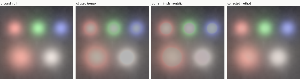
Una escena sintética: tres luces saturadas de un solo canal (discos rojo, verde, azul) y una brillante casi neutra. Ground truth es la escena sin recortar, clipped lo que el sensor registra, previous method el port a Python del módulo à-trous de 2021, corrected method el mismo diseño con la reparación de señal completa descrita justo debajo.
En los discos de un solo canal el resultado corregido trepa de vuelta hacia el color verdadero (p. ej. el disco rojo recupera $\approx 1.7$ frente a $\approx 1.9$ verdadero, con el verde y el azul igualados exactamente) donde el método anterior se queda por debajo del recorte ($\approx 0.9$). El disco neutro totalmente recortado, plano en el recorte tanto en el sensor como en el método anterior, es re-abovedado por el relleno de luminancia compartido (centro $\approx 1.5$ frente a $\approx 1.6$ verdadero) y permanece casi neutro, con su crominancia portada por la difusión del borde.
La reparación de una línea —aplicar el mismo ajuste guiado a la señal completa (baja frecuencia y detalle juntos) de modo que el intercepto porte la media local y un canal quemado pueda subir por encima del recorte (las matemáticas están en las reglas de actualización)— arregla esa clase de fallos, y es el fundamento que todo lo posterior conservó: todos los métodos subsiguientes de este artículo ajustan líneas de color sobre valores completos. Fue necesaria pero no suficiente. Con verdad de referencia contra la que medir —sobre el diseño reparado, reconstruido a resolución completa en torno a una escalera de tamaños de ventana (el anexo del cementerio lo detalla)— cuatro fallos estructurales permanecieron, y dieron forma al método sucesor:
Primero, la escalera de ventanas degenera dondequiera que una ventana vea mayormente datos a nivel de recorte (ventanas finas cerca del borde, ventanas gruesas en lo profundo del agujero), y un ajuste degenerado (covarianza cercana a cero, pendiente cercana a cero) rellena plano, aproximadamente al nivel de recorte. Peor, el traspaso entre escalas consecutivas sigue un contorno de profundidad constante en el agujero, y el desacuerdo de las dos escalas imprime un arco visible a lo largo de él.
Segundo, la amortiguación $\epsilon$ de arriba compite con la varianza local de la guía, de modo que silenciosamente aplasta la pendiente dondequiera que esa varianza sea pequeña —lo cual protege el contenido ruidoso por accidente y aplana gradientes suaves limpios (como el cielo) por el mismo mecanismo. Una constante, dos consecuencias opuestas, ningún valor que sirva a ambas.
Tercero, el sensor no se recorta abruptamente: comprime el último puñado de puntos porcentuales por debajo de la saturación, de modo que la banda de píxeles que la reconstrucción trata como anclajes de confianza se registra sistemáticamente demasiado baja.11 Incluso un oráculo que reconstruyera el interior recortado exactamente se situaría entonces visiblemente más brillante que el anillo sesgado al que debe unirse: la costura está en los datos, no en la estimación, y solo corregir los datos (la inversión del codo) puede eliminarla.
Cuarto, todo el método descansa sobre una hipótesis: los canales vecinos suben y bajan juntos, de modo que un canal recortado es una función afín medible de uno que sobrevivió. Y algún contenido (un cielo cuya tonalidad misma se desplaza, la iridiscencia, una textura de color más fina que la ventana) simplemente no la satisface. Ahí, la guía no contiene información alguna sobre el canal faltante para ningún estimador, así que el diseño debe medir eso ($R^2$) y cambiar por completo la fuente de información: suavidad espacial en lugar de transferencia entre canales.
Arreglar esos casos requirió más que un arreglo: requirió un cambio de paradigma.
El nuevo método: transposición armónica
Esta sección documenta el método que se distribuye hoy: sus premisas, su problema de optimización,
su algoritmo, y cómo la implementación de producción se desvía del prototipo de investigación.
Los resultados medidos, el rendimiento y los hallazgos generales tienen cada uno su propia sección más abajo.
La transposición armónica se distribuye como su propio modo de reconstrucción junto al original
guided laplacians: el método à-trous de 2021 conserva su nombre y diseño históricos —
sin cambios salvo por el arreglo compartido de recolección en bordes, que mejora sus propias puntuaciones — y el nuevo
método es una activación explícita.
El núcleo de reconstrucción es agnóstico al mosaico del sensor y funciona igual en Bayer que en X-Trans, en
el procesador y dentro de un pipe OpenCL, donde cada región recortada se
resuelve en el lado del bus que se midió más rápido
(véase la sección de rendimiento).
Intuición y contexto
La reparación anterior cambia lo que el filtro guiado transfiere; la transposición armónica cambia cómo viaja el modelo. Dondequiera que al menos un canal sobrevivió, la reconstrucción es un problema de regresión, no un problema de relleno (inpainting): los canales válidos son datos medidos, presentes en cada píxel de la zona quemada, y la única incógnita es la relación local (la línea de color) entre ellos y el canal recortado. El método de 2021 — y su reconstrucción corregida sobre la señal completa — evaluaba esa relación dondequiera que una ventana estadística pudiera alcanzar, y unía las evaluaciones entre sí; cada unión era una costura, y las ventanas en lo profundo de un hueco grande no alcanzaban nada en absoluto. La transposición armónica invierte el transporte: ajusta la línea de color una vez, donde los datos la sustentan, luego difunde los coeficientes del modelo — no los valores de píxel — a lo largo de la zona quemada como campos suaves, y solo entonces los evalúa contra los canales supervivientes medidos en cada píxel. Los coeficientes son suaves por naturaleza donde los valores no lo son; las guías reinyectan la estructura a resolución completa en el momento de la evaluación. Por qué esto es una diferencia de tipo y no de grado — y a qué se generaliza — se explica en los hallazgos teóricos.
Todo lo demás que el método de 2021 hacía bien se conserva, sobre una base más sólida: el modelo de línea de color y sus mínimos cuadrados ponderados por ventana (la regresión del filtro guiado), la cúpula biarmónica para la magnitud sin guía, la crominancia llevada como razones acotadas, la preferencia por continuaciones suaves, y la regeneración del grano. Lo que es nuevo, además del transporte: segmentación por región a resolución completa (el coste escala con el área recortada, no con la imagen), una inversión del rolloff del sensor medida que quita el sesgo de la banda cercana al recorte antes de ajustar nada (fallo 3 arriba), ajustes filtrados y confiados según su propia calidad medida $R^2$ (fallo 4), y una regla de diseño aplicada en todas partes, derivada de la ley de energía de costura de los hallazgos teóricos: ningún paso puede transferir el relevo entre estimadores que no concuerdan (fallo 1).
El problema de optimización
Ningún paso ensambla una energía global y llama a un solucionador con nombre, pero cada uno es la regla de actualización local de un problema variacional, y juntos hacen explícito el objetivo. Sobre la región recortada $\Omega$ la reconstrucción minimiza cuatro energías acopladas sobre el modelo.
1. Consistencia afín entre canales. Donde existe una guía válida $g$, cada canal recortado debería ser una función afín de la guía: el filtro guiado es el minimizador exacto de
Ajustar sobre los valores completos $u$ (no el detalle) es lo que hace que el minimizador lleve el promedio local, de modo que $E_{\text{affine}}$ recupera magnitud y textura juntas.310 Este término se confía en proporción a la correlación al cuadrado del ajuste $(R^2)^2$; donde $R^2 \to 0$ el canal se somete en cambio a su propia suavidad de segundo orden (un término biarmónico por canal $\int_\Omega (\Delta u_c)^2, \mathrm{d}\Omega$), de modo que el objetivo nunca premia una línea de color que los datos no sustentan. El elevar al cuadrado agudiza ese compromiso, de manera que una correlación mediocre se apoya en el respaldo suave en lugar de una conjetura discontinua entre canales.
1b. Transporte anisotrópico de coeficientes (la forma distribuida del término 1). El ajuste afín del término 1 define sus coeficientes solo donde una ventana contiene suficientes datos confiables; en el resto de la zona quemada el modelo mismo es la incógnita. El método distribuido lo extiende minimizando una energía de Dirichlet anisotrópica sobre los planos de coeficientes,
donde los anclajes son los ajustes filtrados del término 1 (suficiente masa confiable, $R^2 > 0.25$, pendientes acotadas) y $D$ es el tensor de dirección adaptativo a la varianza del paso 3, construido a partir de la estructura de guía medida: dominado por el gradiente en una rampa limpia de halo (el modelo viaja radialmente hacia adentro desde el borde), dominado por la isofota donde un borde duro cruza la zona (las líneas de color no deben mezclarse a través de la frontera de un objeto). Su ecuación de Euler–Lagrange $\operatorname{div}(D \, \nabla p) = 0$ es el relleno dirigido; con $D = I$ se reduce al relleno armónico simple. La evaluación $\hat u_c = a\,u_{g_1} + b\,u_{g_2} + d$ contra las guías medidas cierra el término: la energía transporta el modelo, y los datos restauran el detalle.
2. Curvatura de magnitud (respaldo). Donde no sobrevive ninguna guía, se pierde el detalle fino pero la forma de baja frecuencia no: debería continuar la curvatura del entorno en lugar de aplanarse. Para un canal parcialmente recortado esto es el término biarmónico por canal $\int_\Omega (\Delta u_c)^2, \mathrm{d}\Omega$ ya invocado arriba. Para el núcleo totalmente recortado se aplica una vez a la luminancia sumada $L_\text{sum} = R+G+B$, una cúpula compartida en lugar de tres divergentes:
anclada al verdadero borde válido del núcleo; su ecuación de Euler–Lagrange $\Delta^2 L = 0$ es el relleno abovedado de arriba.
3. Suavidad de crominancia (respaldo). Donde no sobrevive ninguna guía, las razones reconstruidas $r = \text{RGB}/L_\text{sum}$ deberían ser suaves y coincidir con el borde, opcionalmente sesgadas hacia la planitud:
Su ecuación de Euler–Lagrange es la ecuación de Poisson apantallada que la difusión integra,4 y la recombinación $\text{RGB} = L\cdot r$ cierra el relleno conjunto.
Las energías actúan sobre píxeles complementarios: el término afín donde un canal sobrevive (ponderado por su correlación $R^2$), el término biarmónico por canal donde no, y la cúpula compartida de luminancia más la difusión de crominancia solo en los núcleos totalmente recortados — este último minimizado sujeto a una desigualdad: la razón difundida de un canal recortado nunca puede caer por debajo de su suelo de saturación en el espacio de razones, $r_c \geq c_{0,c}/L_\text{sum}$, lo que convierte el término de crominancia en un problema de obstáculo (la matemática está en la subsección de crominancia). El propio conjunto reconstruible es por canal: $\Omega_c$ contiene los píxeles por encima del umbral de recorte — extendido hacia abajo hasta $0.9$ de él para los canales cuyo rolloff del sensor se activó (la anulación de banda del paso 2), donde el suelo $c_{0,c}$ es la medición corregida por la rodilla en lugar de la lectura saturada. Cada energía se minimiza por su propia etapa: el término afín por los ajustes guiados (una ventana dimensionada al radio de reconstrucción de la región); el término de transporte por la relajación anclada y dirigida del paso 3; los términos de suavidad por sus resoluciones lineales directas. No hay deliberadamente ninguna energía de suavizado posterior que actúe sobre la salida: un diseño anterior planchaba las costuras a posteriori con un regularizador ponderado por incertidumbre, y retirarlo es el punto — las costuras nunca se crean (véase el cementerio). Esta es la misma filosofía de ingeniería que diffuse or sharpen: una pila de reglas de actualización locales, motivadas físicamente, cuyo punto fijo combinado es la reconstrucción, en lugar de un único problema inverso monolítico.
El algoritmo
Todo ocurre sobre el mosaico raw, en RGB lineal referido a la escena (scene-referred), antes del interpolación cromática, y a resolución completa. El método reconstruye cada canal recortado a partir de los canales que sobrevivieron (a lo largo de la línea de color local, confiando en ella en proporción a lo bien que realmente se sostiene), y donde ningún canal sobrevivió reconstruye una cúpula de luminancia conjunta y lleva la crominancia circundante hacia adentro.
La preparación del mosaico — interpolación cromática bilineal a un RGB desechable, normalización local de canales, y la máscara de recorte por canal — se comparte con el método de 2021 y se describe en su sección de algoritmo, con una adición y tres refinamientos. La adición: para los núcleos totalmente recortados se separa una magnitud escalar $L_\text{sum}$ (la luminancia sumada $R+G+B$) de la crominancia $\text{RGB}/L_\text{sum}$ — cada canal dividido por la luminancia sumada, una descripción del color acotada y libre de brillo que este artículo usa consistentemente bajo ese nombre — de modo que las dos pueden reconstruirse por medios diferentes: una cúpula para la magnitud, difusión para la crominancia. Los refinamientos, cada uno rastreado desde un artefacto de borde medido:
- las máscaras son binarias, de principio a fin. El modo de 2021 difumina su máscara; el sucesor mantiene duras todas las máscaras de validez y composición (su único peso suave es la entrega difuminada del núcleo conjunto, paso 7 del algoritmo, que fusiona dos reconstrucciones — nunca reclasifica mediciones). Las máscaras de validez por canal filtran cada ajuste y evaluación, y difuminarlas reclasificaba los fotositos recortados en el borde — cuyos valores raw se sitúan en el umbral de detección, sesgados hacia abajo por el rolloff del sensor — como anclajes válidos en contornos oblicuos, arrastrando la reconstrucción del borde hacia el nivel de recorte (una rampa hundida de $\sim 10$ px contra la verdad de referencia). El peso de composición es un interruptor duro: los fotositos válidos conservan su medición exactamente, los fotositos recortados toman la reconstrucción pura (se midió que un alfa difuminado no cambia nada una vez que los dos arreglos de esta lista están en su sitio — la retirada se documenta en el cementerio).
- los valores raw recortados son suelos, nunca objetivos de fusión. En los fotositos recortados la lectura raw es una cota inferior, no una medición: el compuesto escribe $\max(\text{raw}, \text{reconstruction})$, nunca una fusión hacia la lectura sesgada (la antigua fusión difuminada imprimía una caída en forma de V a través del valor raw en cada contorno).
- los bordes se reflejan (espejo). El anillo de borde de la recolección bilineal solía copiar el fotosito central en los tres canales y basar los tres indicadores de recorte en el propio canal del centro — corrompía las guías y punteaba las máscaras a lo largo de la primera y última filas y columnas, lo que anclaba los ajustes de la fila de borde al nivel de recorte. La indexación de vecinos reflejada (el patrón Bayer es 2-periódico, así que reflejar preserva el color de cada vecino) restaura la lógica interior en los bordes; este arreglo se comparte con el modo de 2021.
Cada escena de verdad de referencia mejoró en ambas métricas solo con estos tres refinamientos — el error del cielo con rolloff cayó en un tercio — porque los anillos de borde del banco de pruebas son exactamente donde los anclajes sesgados solían filtrarse.
El objetivo conceptual de la reconstrucción puede enunciarse en una frase: dondequiera que al menos un canal sobrevivió, la reconstrucción es un problema de regresión, no un problema de relleno (inpainting): los canales válidos son datos medidos, presentes en cada píxel de la zona recortada, que llevan la verdadera estructura de la escena. La única regla de diseño del algoritmo, aprendida a las malas, es que ningún paso puede transferir el relevo entre estimadores que no concuerdan (la ley de energía de costura de los hallazgos teóricos). Por tanto cada etapa de abajo está libre de costuras por construcción, o bien quita el sesgo de los datos para que los estimadores concuerden.
El procedimiento paso a paso, tal como está implementado en process_harmonic_bayer (y su gemelo X-Trans):
Los números en el gráfico se refieren a los pasos detallados debajo de él.
flowchart TD
  subgraph P ["once per image"]
    direction TB
    A["raw mosaic"] --> B["1 · interpolate
+ clip masks"]
    B --> K["2 · knee inversion"]
    K --> S["1 · depth map
+ segmentation"]
  end
  subgraph R ["for each clipped region"]
    direction TB
    CF["3 · colour-line fits
(magnitude + texture)"] --> HF["4 · fine-detail refit"]
    HF --> SD["5–6 · floors
+ self-dome"]
    SD --> JC["7 · all-clipped core"]
    JC --> AN["8 · chrominance coherence"]
  end
  S --> CF
  AN --> O["remosaic + composite"]
1. Detección, interpolación, segmentación. El mosaico raw de la matriz de filtros de color se interpola bilinealmente, con indicadores de recorte por canal levantados en $0.995\,c$ para un nivel de recorte $c$ y una máscara de validez binaria por canal; la transformada de distancia euclidiana da luego a cada píxel su profundidad $\delta$ dentro de la zona recortada, y la segmentación por componentes conexas agrupa los píxeles recortados en regiones, cada una llevando su radio de reconstrucción de la transformada de distancia.
2. Inversión del rolloff (rodilla) del sensor. Los sensores reales comprimen el último pequeño porcentaje por debajo de la saturación, así que la banda cercana al recorte $[0.8\,c, 0.995\,c)$ contiene valores sesgados hacia abajo. (La banda se corta generosamente: en sensores que recortan de forma dura en lugar de hacer rolloff, la garantía de no-operación de abajo hace que el ancho extra sea gratuito.) La reconstrucción extrapola estimaciones sin sesgo sobre esta banda, así que las dos no concuerdan en el contorno de detección: una costura que ninguna ponderación puede eliminar. El arreglo quita el sesgo de los datos mismos: una regresión conjunta por ventana predice cada valor de banda a partir de los canales plenamente confiables, los pares (medido, predicho) se agrupan en 24 contenedores (bins) sobre la banda, y el levantamiento mediano por contenedor se acepta solo cuando es estadísticamente significativo — mediana por encima del doble de su error estándar, una compuerta de confianza del $\approx 95\,\%$, con al menos 100 votos para que la propia estimación del error sea estable; 24 contenedores es tan fino como se puede cortar la banda manteniendo cada contenedor poblado:
donde $k$ es la compresión desconocida del sensor, así que $\hat{k}^{-1}$ es la
corrección estimada — la función que toma un valor medido $v$ de la banda y devuelve
lo que el sensor debería haber registrado. Los $v_i$ son todos los píxeles de banda medidos cuyo valor
cae en el mismo contenedor que $v$; cada $\hat v_i$ es lo que la
regresión de línea de color predice que ese píxel debería ser, juzgando a partir de sus canales vecinos
plenamente confiables. Su diferencia $\hat v_i - v_i$ es el voto de un píxel sobre cuánto
subregistró el sensor en ese nivel, y la corrección del contenedor es la mediana de sus votos —
robusta frente a los valores atípicos que una media seguiría. La curva resultante se hace luego monótona y
solo-ascendente. En datos recortados de forma dura (sin sesgo) cada mediana de contenedor es cero dentro del
ruido, así que la corrección tiene una garantía de no-operación, verificada bit-exacta en los cuatro casos sintéticos
de recorte duro, mientras que en pk1synth (la única escena sintética generada con un rolloff analítico del
sensor, de modo que su verdad de referencia traza la rodilla real) la estimación a ciegas coincide con la curva
verdadera con un error cuadrático medio de $7\cdot10^{-4}$ en el canal verde y $1.8\cdot10^{-3}$
en el rojo, más escaso:
La anulación de banda. El levantamiento restaura el nivel de la banda, pero un mapa de valores no puede restaurar una pendiente que el sensor nunca registró: donde la compresión aplanó la banda hasta casi una constante, la banda levantada es también casi una constante, y su unión con la reconstrucción ascendente imprime un fino doble contorno bajo la ampliación de bordes (la banda es medibliemente $7$–$14\times$ más plana que la verdad de referencia, flanqueada por dos picos de gradiente). La información no se pierde, sin embargo — las guías están sin recortar a través de la banda y llevan la pendiente verdadera. Así que para cada canal cuyo rolloff se activó, la detección se extiende por debajo del umbral hacia la banda profunda: esos píxeles se reconstruyen mediante el modelo de línea de color como cualquier píxel recortado, con su medición levantada por la rodilla como su suelo de saturación por píxel, y los ajustes se anclan en datos corregidos por la rodilla por debajo de la banda. El suelo hace la anulación conservadora por construcción — en imágenes reales ruidosas el modelo rara vez excede la medición levantada, y la salida se mantiene idéntica píxel a píxel; en la escena de banco con rolloff, donde el modelo genuinamente conoce la pendiente, el error de la zona cae otro factor de cinco cuando la anulación acierta (RMSE $0.012 \to 0.0025$ medido entonces; $0.0053$ en la compilación distribuida, después de que las rondas de composición posteriores tomaran sus propios mordiscos) y el perfil de gradiente del contorno se vuelve indistinguible de la verdad de referencia. Los canales sin un rolloff medido mantienen la detección simple: en sensores de recorte duro la banda es un dato fiable y permanece anclada.
3. El campo de coeficientes. Para cada canal recortado $v$ con guías $u_1, u_2$, se calcula un ajuste de mínimos cuadrados ponderado por ventana a una única escala $\sigma = \operatorname{clip}(r/6, 8, 64)$ (con $r$ el radio de reconstrucción de la región — el soporte $\pm 3\sigma$ de la ventana abarca entonces el radio, así que hasta el ajuste del píxel más profundo alcanza datos válidos; el suelo mantiene suficientes muestras para un ajuste estable en regiones diminutas, y el tope acota el coste de las enormes), sobre los píxeles donde los tres canales son válidos:
donde $x$ es el píxel cuyo modelo local se está construyendo e $y$ recorre sus vecinos. La ventana $G_\sigma(x-y)$ es una gaussiana que pondera los vecinos por distancia (peso completo cerca, desvaneciéndose a lo largo de aproximadamente $\sigma$ píxeles), y $w(y)$ es la máscara de confianza — uno en los píxeles donde los tres canales tienen mediciones reales, cero en el resto, así que los píxeles recortados nunca votan. La primera línea pregunta, en cada $x$: ¿qué pendientes $a, b$ sobre las dos guías y qué desplazamiento $d$ explican mejor el canal recortado en el vecindario confiable? La segunda línea entonces usa ese modelo local: la estimación $\hat v(x)$ lee las dos guías en el propio $x$ y las mapea a través de la relación ajustada. En la práctica la minimización nunca se corre por píxel — se resuelve a partir de diez planos de momentos difuminados (un recuento de masa confiable, tres medias, seis segundos momentos, recolectados en tres difuminados de cuatro canales) mediante las ecuaciones normales $2\times2$. Los momentos se acumulan en torno a la media por región de cada canal: en aritmética de flotantes la forma cruda $E[u^2] - E[u]^2$ se cancela catastróficamente en contenido suave (la media al cuadrado empequeñece la varianza) y la división del ajuste amplifica los dígitos supervivientes hasta un ruido de pendiente dependiente del dispositivo — centrar elimina la cancelación, y las pendientes y $R^2$ son invariantes bajo el desplazamiento mientras que la ordenada al origen se desplaza de vuelta justo después del ajuste. El sistema se resuelve con un amortiguamiento de Tikhonov (cresta) relativo $\lambda = 10^{-3}\,(\operatorname{var} u_1 + \operatorname{var} u_2)/2$ que escala con la señal en lugar de comerse pendientes débiles-pero-reales. El $10^{-3}$ es el factor más pequeño que estabilizó las ventanas degeneradas en el banco — cualquier valor mayor empieza a aplanar pendientes reales.
La novedad es lo que pasa a continuación: en lugar de evaluar cada píxel con el ajuste que su propia ventana pudiera alcanzar (el modo de la escalera), los propios planos de coeficientes se difunden a través de la zona recortada, dirigidos por la estructura de guía medida, y solo entonces se evalúan contra las guías medidas. Los coeficientes son suaves por naturaleza donde los valores no lo son: difundirlos transporta el modelo a la zona, y la evaluación restaura la estructura local completa llevada por los canales válidos. Sin escalas, sin compuertas de profundidad, sin escrituras de conjuntos de nivel (sin anillos de igual profundidad estampados por separado) — sin costuras, por construcción. Este transporte del modelo en lugar del contenido es la idea más transportable del artículo, y cómo difiere en tipo del propio difuminado de coeficientes del filtro guiado se expone en Tres resultados que creemos generales. Un píxel califica como anclaje de difusión solo si su ventana contenía suficiente masa confiable y su ajuste es cuerdo: el $R^2$ del ajuste, el coeficiente de determinación, es la fracción de la varianza local del canal que la línea de color explica (1 significa que las guías predicen el canal perfectamente, 0 significa nada en absoluto), y los anclajes requieren $R^2 > 0.25$ con pendientes acotadas. Ambas compuertas están calibradas a partir de mediciones, no del gusto: el contenido sin línea de color en absoluto aún puntúa $R^2 \approx 0.25$–$0.6$ (frente a $\approx 0.9$ donde la línea de color es real), así que la compuerta solo rechaza ajustes peores que la pura decorrelación — accidentes numéricos, no modelos débiles; y las pendientes físicas de línea de color están acotadas por las razones de saturación de los canales (por debajo de $4$ en cada cámara medida), así que la cota $|a| < 64$ se sitúa un orden de magnitud por encima de cualquier cosa física, y solo las ventanas degeneradas de varianza casi nula — cuyas pendientes explosivas envenenarían la frontera de difusión — llegan a activarla. La difusión es un relleno de Jacobi de grueso-a-fino: cada incógnita se reemplaza repetidamente por el promedio que sus vecinos implican. Tres términos llevan todo el esquema:
- Celda. El relleno no corre por píxel. Los planos de coeficientes viven en una rejilla gruesa de paso $\sigma/4$ (fijada a como mucho $8$ px), y una celda es un nodo de esa rejilla — un bloque de píxeles de tamaño $\sigma/4$. Los coeficientes salen de ventanas de ajuste de ancho $\sigma$, así que cuatro celdas por $\sigma$ las sobremuestrean, y la fijación del paso acota el error final de sobremuestreo bilineal.
- Anclaje. Una celda cuya ventana de ajuste pasó las compuertas de confianza de arriba — contiene un coeficiente realmente medido sobre datos válidos.
- Fijado (pinned). Los barridos tratan los anclajes como datos de frontera fijos y solo reescriben las celdas desconocidas entre ellos.
Esta forma se elige por robustez. Un gradiente conjugado en flotantes sobre el sistema puramente armónico casi singular diverge estocásticamente cuando la zona alcanza la frontera de la región. Jacobi con anclajes fijados no puede: cada actualización es un promedio de vecinos, así que la relajación obedece el principio del máximo — ninguna incógnita puede jamás salir del rango de los valores de anclaje.
La convergencia viene de la profundidad de la pirámide, no del número de barridos. El nivel más grueso parte de una media de anclaje plana — el estado más lejano posible de la solución — y el modo de error más lento de Jacobi sobre un hueco de $N$ celdas de ancho decae en $\mathcal{O}(N^2)$ barridos. Así que la pirámide sigue dividiendo por la mitad hasta que el lado largo de la rejilla más gruesa sea a lo sumo $8$ celdas ($8^2 = 64$ barridos para relajar, cómodamente dentro del presupuesto), y cada nivel corre luego los mismos $100$ barridos planos — los niveles más finos solo corrigen el error local de interpolación. Una pirámide más superficial con un número fijo truncaba medibliemente el relleno en huecos profundos — los números están en los resultados generales de abajo.
Note
Esta es la única pirámide restante del método, y pertenece al relleno — el transporte de coeficientes ya ajustados. No está relacionada con las ventanas de ajuste, que usan una única $\sigma$ derivada del radio por región (las ventanas multiescala existen solo dentro del estimador de rodilla), y no es la retirada pirámide de croma en forma de traza del núcleo totalmente recortado, que la resolución directa en forma de divergencia reemplazó y que sobrevive solo como respaldo para núcleos por encima de $2^{14}$ incógnitas.
El transporte mismo tampoco es uniforme: está dirigido por la estructura de guía medida. Un plano de dirección $L_\text{mean}$ — la media de los canales válidos dondequiera que al menos uno sobreviva, la media de la meseta plana en el núcleo totalmente recortado (donde el tensor degenera entonces a la identidad); esta es una luminancia diferente de la magnitud sumada $L_\text{sum}$ que usan la cúpula y las razones — se submuestrea a cada nivel de la pirámide, y los promedios de vecinos se ponderan por el tensor anisotrópico
donde $g$ es la dirección unitaria del gradiente de $L_\text{mean}$ (cuesta arriba), $t$ la dirección unitaria de la isofota, y $\langle\lVert\nabla L_\text{mean}\rVert\rangle$ la magnitud del gradiente promediada sobre la región — la normalización que hace el amortiguamiento independiente de la exposición — (a lo largo de las líneas de nivel), y $c_2$ el mismo amortiguamiento de cruce de bordes que el paso de crominancia del paso 8. Normalizar el gradiente por su propia media regional hace ese amortiguamiento sin escala — solo los gradientes muy por encima de la media del halo se leen como fronteras, y el $4$ fija cuán suave es la lectura. El peso de fusión $m \in [0, 1]$ es la probabilidad de borde, medida a partir de la varianza por ventana corregida por tendencia de $L_\text{mean}$:
donde $\operatorname{var}_w$ y $\bar L_\text{mean}$ son la varianza y la media por ventana del plano de dirección, y el término $\tfrac{4}{3}\lVert\nabla L_\text{mean}\rVert^2$ resta la varianza que la rampa local explica: una rampa pura de pendiente $\nabla L_\text{mean}$ vista a través de una ventana de varianza espacial $\sigma_w^2$ tiene una varianza de intensidad $\sigma_w^2 \lVert\nabla L_\text{mean}\rVert^2$, y la ventana aquí (dos pasos de caja $3\times3$) tiene $\sigma_w^2 = 2 \cdot \tfrac{2}{3} = \tfrac{4}{3}$ por eje. Un gradiente de halo suave, por empinado que sea, no deja por tanto ningún residuo, mientras que un borde duro deja una varianza que ninguna rampa puede explicar. El umbral $k$ — el contraste relativo por encima del cual la textura residual se lee como una frontera — es la única constante del transporte que no pudo derivarse, así que se calibró mediante un barrido fino empírico sobre las seis escenas de verdad de referencia: cada escena se mantiene en o por debajo del error isotrópico sobre todo el rango $k \in [0.14, 0.25]$ (el diseño no es frágil ante ello), y $k = 0.15$ es el valor que mejora cada escena simultáneamente y se lleva la victoria en oclusión con margen. Los dos límites de $m$ se leen naturalmente. En una rampa limpia de halo ($m \to 0$), $D \to g\,g^{\top} + c_2\,t\,t^{\top}$: el modelo viaja radialmente, a lo largo de la rampa de brillo desde el borde hacia adentro, donde su información realmente vive. Donde un borde duro cruza la zona quemada ($m \to 1$), $D \to t\,t^{\top} + c_2\,g\,g^{\top}$ con $c_2$ pequeño: el transporte corre a lo largo de la frontera y se niega a cruzarla — un borde dentro de la zona significa que el contenido más allá sigue otra línea de color, y mezclar los dos modelos a través de él es exactamente el fallo de oclusión que documenta el cementerio. La discretización usa el esténcil que preserva la no-negatividad compartido con la difusión del paso 8 (los ocho pesos de vecinos $\geq 0$), así que el relleno dirigido sigue siendo una combinación convexa de sus anclajes: el principio del máximo sobrevive a la dirección. Un suelo de peso de $10^{-4}$ mantiene cada celda conectada donde el tensor colapsa a casi cero; cuatro órdenes de magnitud por debajo de los pesos de trabajo, nunca compite con la dirección. Los píxeles con una única guía superviviente reciben el mismo tratamiento con un ajuste de una guía.
Una sutileza de ordenamiento completa el paso. El canal más profundo — el que tiene más fotositos recortados, cuya zona contiene los núcleos donde varios canales están quemados a la vez — no se evalúa de inmediato: sus coeficientes difundidos se guardan, y la evaluación corre al final, después de que los otros canales recortados hayan sido reconstruidos, así que cada guía que lee es una superficie continua. Evaluarlo contra una guía que salta de valores medidos a una meseta de recorte imprimiría el propio contorno de recorte de esa guía en el resultado como un arco visible. En lo profundo del núcleo, donde esas guías son ellas mismas reconstrucciones (así que cada salto compone error), la estimación se funde de vuelta hacia el ajuste directo de una guía mediante un peso suave — peso suave por campos suaves no deja ningún conjunto de nivel que imprimir.
La calidad del ajuste $R^2$ se difunde junto a $(a, b, d)$ como un cuarto plano, sobre el conjunto de anclajes más amplio de solo-masa (se mantiene acotada incluso donde el ajuste no lo hace).
4. Guiado híbrido de banda laplaciana de las altas frecuencias. El ajuste sobre la señal completa transfiere la textura fina de las guías con las ganancias que implica la covarianza total; donde la línea de color es débil esa textura no pertenece al canal reconstruido. La estimación se divide en $\sigma/4$ y su banda de detalle se reconstruye a partir de dos fuentes candidatas: la transferencia amortiguada (las altas frecuencias de la señal completa escaladas por el $R^2$ difundido) y una línea de color dedicada de banda de detalle (el homónimo del método de 2021, de vuelta), ajustada sobre los planos de alta frecuencia con ganancias encogidas por $R^2$ (en una banda de media cero, el encogimiento es el estimador correcto: no hay magnitud que perder, solo ruido que no imprimir). Las dos se fusionan por probabilidades cuadráticas de energía mínima,
que no necesita ningún discriminador de contenido: una ganancia de ventana mixta que falla en el borde de un objeto aparece como un pico local de energía de alta frecuencia, así que el fallo se detecta a sí mismo y el camino amortiguado toma el relevo exactamente ahí. Esto es lo que elimina el último residuo de la escena de rolloff (su puntuación de exceso de bordes cae de 1.48 a 0.94 frente a un suelo de verdad de referencia de 0.69: el ruido de la banda descomprimida ya no se imprime — los arreglos de sesgo de borde de la compilación final lo llevan a 0.74, y la anulación de banda del paso 2 a 0.64, la tabla de resultados) mientras mejora los casos texturados que el ajuste puro de banda de detalle solía romper.
5. Suelo de saturación suave. El suelo físico (un canal recortado es al menos su lectura saturada $c_0$) se aplica como una restricción redondeada, $\tfrac{1}{2}\big(e + c_0 + \sqrt{(e - c_0)^2 + (0.02\,c_0)^2}\,\big)$: el $\max(e, c_0)$ duro imprime el contorno vinculante como un borde dondequiera que una predicción débil oscila alrededor de la saturación. El ancho de transición $0.02\,c_0$ es el dos por ciento del valor saturado — por debajo de cualquier cosa visible, pero lo bastante ancho para que el gradiente de la restricción nunca salte.
6. Autocúpula acoplada al tono, controlada por profundidad. Donde el modelo es dudoso y el píxel es poco profundo, una autocontinuación suave toma el relevo, construida acoplada al tono (los canales están acoplados a través de una crominancia compartida, así que el tono percibido no puede desviarse): una cúpula de luminancia biarmónica compartida por una crominancia rellenada armónicamente, nunca tres canales independientes, así que el respaldo no puede dividir el tono hacia verde/magenta (el fallo que mantuvo deshabilitado a su ancestro por canal). El peso de entrega es:
donde $\delta$ es la profundidad del píxel dentro de la zona recortada (su distancia al píxel válido más cercano), $\sigma$ la escala de ajuste, y $S$ un smoothstep, una rampa suave de 0 a 1 entre los dos umbrales, aquí mapeando la calidad del ajuste por debajo de $0.4$ a “dudoso” y por encima de $0.85$ a “confiable”. Los bordes de la banda y la escala de profundidad $1.5\sigma$ se afinaron en el banco de verdad de referencia; la escala de profundidad ata el alcance de la cúpula al propio alcance de la ventana de ajuste, así que la entrega ocurre donde el ajuste genuinamente se queda sin muestras. Los dos factores responden a dos preguntas diferentes: $R^2$ pregunta ¿es la línea de color real aquí, y la profundidad pregunta ¿es la cúpula confiable aquí (la extrapolación biarmónica es excelente cerca del borde y se degrada con la distancia). La profundidad es la única señal que encontramos cuyas distribuciones realmente separan las zonas profundas correlacionadas del contenido superficial decorrelacionado (véase el cementerio); los interiores profundos siempre se quedan en el campo de coeficientes.
7. Núcleo conjunto, difuminado. Los píxeles totalmente recortados no tienen guías: la cúpula de luminancia biarmónica compartida y la difusión apantallada de crominancia de borde de la reconstrucción los reconstruyen, sin cambios — pero el compuesto ahora se difumina sobre una máscara de todo-recortado difuminada en lugar de escribirse a través de una dura. La cúpula y la crominancia difundida son ambas válidas más allá de la frontera del hueco, así que fusionarlas en los canales recortados del anillo circundante es continuo en el espacio sin coste alguno para el núcleo mismo.
8. Chrominance coherence. The structure-steered chrominance of the all-clip core is now solved directly. The unknown $u$ is each chrominance plane in turn ; the equation is $\mathrm{div}(D\,\nabla u) = 0$, the steady state of the anisotropic diffusion of the theory section and, equivalently, the exact minimizer of its weighted smoothness energy $\int_\Omega \nabla u^\top D\,\nabla u\,\mathrm{d}\Omega$, with the coefficient-field results as Dirichlet anchors, fixed boundary values the solve must honour. The tensor is built from the recovered luminance (the reconstruction’s own output, smoothed by two box-blur passes) : with $g$ the unit gradient of that smoothed luminance and $t = g^\perp$ the isophote direction,
es decir: conductancia uno a lo largo de las isofotas, amortiguada exponencialmente a través de ellas, con el amortiguamiento normalizado por la propia magnitud media del gradiente de la imagen $\langle \lVert \nabla L_\text{sum} \rVert \rangle$ para que la dirección no dependa de la exposición (este tensor lee la luminancia sumada recuperada — la forma gemela del relleno de coeficientes lee $L_\text{mean}$). La discretización es el esténcil que preserva la no-negatividad de Weickert, una M-matriz simétrica definida positiva, así que el principio del máximo discreto se cumple por construcción: las razones difundidas nunca pueden sobrepasar la crominancia del borde, cosa que el flujo explícito anterior sí podía. La factorización de Cholesky dispersa factoriza el núcleo una vez y retro-sustituye los tres canales. (Una comparativa de solucionadores hay detrás de esta elección: véase el cementerio para el fallo instructivo de la otra formulación exacta.) El remosaicado final compone la salida a partir de la CFA corregida por la rodilla, así que la banda sin sesgo llega al archivo, no solo a los ajustes.
Las reglas de actualización
El problema de optimización enuncia lo que la reconstrucción minimiza y el algoritmo narra sus etapas; la discusión de abajo analiza el diseño — qué representan los parámetros, cómo se afinaron, cómo se relacionan las elecciones con la teoría establecida. Lo que un implementador que parte de cero necesita son las actualizaciones de señal reales: qué ecuación escribe qué plano, en qué orden. Aquí está el catálogo completo, en orden de ejecución, para una región. Planos: estimaciones por canal $u_c$ (inicializadas a la interpolación bilineal del mosaico medido, corregida por la rodilla), validez binarias $v_c$, suelos por píxel $c_{0,c}$ (la medición corregida por la rodilla de cada píxel reconstruible), luminancia sumada $L_\text{sum} = \sum_c u_c$ y razones $r_c = u_c / L_\text{sum}$ (el plano de dirección $L_\text{mean}$ de la regla 1 es la media de canales válidos, una cantidad separada).
1. Ajustar y transportar la línea de color (pasos 2–3 del algoritmo). El ajuste es sobre los valores de píxel completos — nunca el detalle con la media restada — y usa solo las muestras donde los canales involucrados son válidos. En la forma de una guía, sobre la ventana gaussiana $\omega$:
con $\varepsilon$ un amortiguamiento de Tikhonov relativo que protege la división donde la guía es plana; la forma de dos guías resuelve las ecuaciones normales $2\times2$ análogas para $(a, b, d)$ a partir de los diez planos de momentos difuminados por gaussiana. La pendiente no se recorta por signo (una revisión temprana de la escalera la recortaba; los ajustes distribuidos están protegidos en cambio por las compuertas de anclaje $R^2 > 0.25$ y $|a| < 64$). Dos compuertas más que un implementador no debe saltarse: las ventanas de ajuste se ponderan por una afinidad de luminancia suave $\min(L_\text{sum} / 0.35\,\bar L_\text{sum}^{\,\text{rim}}, 1)^2$ — las muestras mucho más oscuras que el borde (oclusores) apenas votan — y una ventana solo ancla el transporte donde su masa ponderada excede tanto un suelo absoluto (0.05) como un cuarto de su masa válida no ponderada, así que las ventanas ocluidas ceden al relleno en lugar de ajustar al oclusor. Como el ajuste es sobre valores, la ordenada al origen lleva el promedio local del color: la predicción hereda el nivel de los datos válidos circundantes, no solo su textura, así que donde la guía sigue subiendo hacia la alta luz la estimación la sigue — por encima del valor de recorte. En la práctica el ajuste nunca se corre por píxel: los momentos son planos de producto difuminados por gaussiana, centrados en las medias válidas por región contra la cancelación de flotantes.
Note
Ajustar a partir de las muestras válidas únicamente es esencial. Las muestras recortadas están fijadas en el punto blanco; incluirlas aplanaría la pendiente observada, y el modelo reproduciría el valor recortado en lugar de extrapolar más allá de él. Esta es la única sutileza que separa una reconstrucción funcional de una que meramente repinta el recorte.
Filtra los anclajes ($R^2 > 0.25$, pendientes acotadas, masa confiable), luego difunde cada plano de coeficientes mediante barridos de Jacobi anclados sobre la rejilla gruesa — la actualización de un barrido en una celda no-anclaje $i$, con los ocho pesos de Weickert $w_{ik}$ del tensor $D$:
anclajes mantenidos fijos, 100 barridos por nivel de pirámide, el nivel más grueso sembrado con la media de anclaje y cada nivel más fino sembrado por sobremuestreo bilineal de la solución más gruesa; misma actualización para $b$, $d$ y $R^2$. Luego evalúa el modelo transportado contra las guías medidas, en cada píxel donde el objetivo está recortado y ambas guías son válidas:
Los píxeles con una única guía válida toman la misma actualización del ajuste de una guía $u_c \leftarrow a\, u_g + d$. La evaluación del canal más profundo se difiere hasta que los otros canales recortados se reconstruyen, así que sus guías son superficies continuas.
2. Reconstruir las altas frecuencias (paso 4). Divide $u_{g}$ en baja frecuencia $\bar u_g$ (gaussiana en $\sigma/4$, con suelo en 2 px — los momentos usan la $\sigma$ del ajuste, la división de banda no) y detalle $u_g - \bar u_g$; forma los dos candidatos — la transferencia de guía $h_g = a\,(u_{g_1} - \bar u_{g_1}) + b\,(u_{g_2} - \bar u_{g_2})$ y el autodetalle amortiguado $h_d = R^2 (u_c - \bar u_c)$ — y fusiónalos por probabilidades cuadráticas de energía mínima sobre sus energías locales (difuminadas por gaussiana) $e_g, e_d$, exactamente como enuncia el paso 4 (un interruptor duro reintroduciría una costura de relevo):
3. Suelo de saturación suave (paso 5), en todas partes donde un canal es reconstruible, con $w = 0.02\, c_{0,c}$:
4. Autocúpula controlada por profundidad (paso 6). Resuelve una continuación biarmónica compartida de la luminancia sobre el hueco, $\Delta^2 L_b = 0$ con $L_b$ anclado en el borde (Cholesky disperso directo sobre el bilaplaciano discreto de 13 puntos, rejilla gruesa — el mismo solucionador que la sección de implementación documenta), separa su crominancia del borde ($\bar r_c$, relleno armónico), y fusiona por la fracción de cúpula $f$:
con $\delta$ la profundidad del píxel dentro de la zona recortada (su distancia al píxel válido más cercano — el único significado que $\delta$ lleva en este artículo).
5. Núcleo totalmente recortado (pasos 7–8), sobre los píxeles donde ningún canal sobrevivió. Magnitud: la cúpula biarmónica $\Delta^2 L = 0$ anclada en el anillo (ya reconstruido). Crominancia: primero el relleno de borde de Poisson apantallado por canal, $(\Delta - \lambda)\, r_c = -\lambda\, \bar c_c$ con $\bar c_c$ la cromaticidad válida media de la región rellenada y $\lambda$ la reacción de color plano (resolución dispersa directa, factorización compartida); luego el paso dirigido por estructura. Su forma primaria es la resolución exacta en forma de divergencia del paso 8 (laplaciano de grafo de 8 vecinos ponderado por bordes, factorización dispersa directa); los núcleos por encima de $2^{14}$ incógnitas toman la pirámide explícita en forma de traza en su lugar — pasos bajo el obstáculo, iterados 240 veces por nivel:
seguido de un pulido proyectado de 60 barridos a resolución completa (controlado por actividad: corre solo donde algún píxel realmente se sitúa sobre su suelo). Reensamblaje, por píxel del núcleo totalmente recortado — los únicos píxeles que este paso escribe; los píxeles parcialmente recortados fueron resueltos por las reglas 1–4 y actúan como sus anclajes:
con suelo suave como en la regla 3. (El código también lleva una rama de transferencia de magnitud para píxeles parcialmente válidos, un remanente de la era de la escalera que la construcción de anclajes hace inalcanzable — documentado aquí para que nadie lo transcriba.)
6. Grano y compuesto. Añade el grano poissoniano de la siguiente subsección donde se solicite, luego reescribe a través del interruptor duro: los fotositos reconstruibles toman $\max(\text{raw}, u_c)$, los fotositos válidos conservan su medición intacta.
Todo lo demás en el pipeline — la estimación de la rodilla, la segmentación, el rellenado — prepara entradas para estas seis actualizaciones; nada más escribe un píxel.
Discusión
Los operadores que compone el algoritmo no son arbitrarios: cada uno es el estimador que su término de energía prescribe, y cada uno lleva propiedades medibles en las que el diseño se apoya. Esta subsección las deriva, y cierra con el estudio de parámetros que dimensiona todo el método — cuán lejos debería alcanzar una reconstrucción.
Confiar en la guía
El préstamo de línea de color es solo tan bueno como la suposición que hay detrás: que el canal recortado y su guía están, localmente, relacionados de forma afín. En una superficie natural lo están; en contenido patológico (gradientes independientes por canal, o una frontera entre dos materiales de colores diferentes) no lo están, y forzar el préstamo pintaría estructura que no pertenece. El ajuste mismo informa de cuánto confiar en él: $R^2$ (definido junto con el ajuste, en las reglas de actualización) es la fracción de la varianza local del canal que la línea de color explica — $1$ donde el modelo se sostiene, $0$ donde el préstamo carece de sentido.
Así que el método nunca conmuta entre el relleno entre canales y el de un solo canal — los fusiona por confianza, cayendo de vuelta a extender el propio gradiente del canal recortado hacia adentro (relleno biarmónico por canal, anclado en el verdadero borde válido de ese canal) a medida que la línea de color se debilita. El peso de fusión es la confianza al cuadrado $W_e = (R^2)^2$, y el exponente es una elección medida, no del gusto. Sobre los píxeles recortados, $R^2$ separa los dos regímenes solo con un margen suave: promedia $\approx 0.9$ en contenido de tipo natural, $\approx 0.65$ en contenido decorrelacionado, y las dos distribuciones se solapan en $\sim15\%$ — y ningún estadístico más barato lo hace mejor (se midió que tanto la estabilidad de pendiente entre escalas como la concordancia entre guías separan peor, así que $R^2$ es el techo honesto). Usado linealmente, el caso decorrelacionado aún tomaría $\sim65\%$ de una estimación entre canales que es a la vez errónea y — porque la selección dura de guía se invierte ahí — discontinua. Elevar al cuadrado separa los regímenes: $0.9^2 \approx 0.81$ apenas mueve el caso confiable, mientras que $0.65^2 \approx 0.42$ reduce a la mitad el no confiable, así que los píxeles decorrelacionados se apoyan en el relleno suave de gradiente propio. Sin embargo, como el margen es suave, una costura tenue aún sobrevive en el contenido más adversarial: elevar al cuadrado no puede ocultar del todo una discontinuidad en la cantidad que pondera, y ese residuo es para lo que existe la regla de diseño de nunca-crear-costuras (véase el cementerio).
Donde ningún canal sobrevive no hay guía ni $R^2$ que ponderar, así que la reconstrucción transfiere el relevo al núcleo conjunto de la siguiente sección. La fusión está así controlada por la validez de guía y ponderada por la correlación al cuadrado, no por un recuento duro de canales recortados: un mecanismo abarca todo el rango desde un recorte de un canal (mayormente entre canales) pasando por un recorte de dos canales (el canal superviviente guía) hasta un núcleo totalmente quemado (la cúpula conjunta). Esto es lo que hace que el método se degrade con gracia a medida que la correlación entre canales cae: en las imágenes de prueba de tipo natural el término entre canales domina, en los gradientes aleatorios adversariales la autoextensión toma el relevo, y la reconstrucción nunca fabrica una línea de color que no está ahí. Es la correlación, no el número de supervivientes, lo que decide si se puede confiar en una guía — un píxel con dos supervivientes en contenido decorrelacionado no está mejor guiado que un píxel con un superviviente en una línea de color limpia.
Rellenar huecos sin superviviente
Donde todos los canales recortan, no se puede ajustar ninguna línea de color: el detalle fino de la alta luz y su pico exacto se pierden genuinamente. Pero aún se pueden rescatar dos cosas del entorno, siempre que se reconstruyan conjuntamente: la curvatura de magnitud de baja frecuencia del hueco y su crominancia.
La jugada ingenua es abovedar cada canal de forma independiente: correr el autorelleno biarmónico por canal del respaldo de confianza, ahora sin ponderar, sobre los tres canales. Falla de una forma instructiva. Como los canales recortan a radios diferentes (cada uno tiene su propio nivel de blanco, y una alta luz casi neutra los cruza por turnos), cada canal se abovedar desde un borde a una distancia diferente del centro, y las tres cúpulas alcanzan alturas diferentes. El último canal en recortar se satura plano justo en su borde, así que lleva casi ninguna pendiente hacia adentro y su cúpula apenas sube, mientras que el primer canal en recortar se abovedar a lo largo de un radio ancho y sube empinadamente. El núcleo por tanto se desvía fuera de tono: un sol neutro quemado sobre un cielo naranja se reconstruye como un disco amarillo, porque el azul (el último en recortar aquí) colapsa mientras el rojo se sobrerrecupera. Tres cúpulas 1-D de aspecto correcto, un color equivocado.
El arreglo es separar lo que se comparte de lo que no. La magnitud es común a los tres canales (todos están brillantes porque la misma luz los desbordó), así que se reconstruye una vez, como una única cúpula. La crominancia varía suavemente y se lleva hacia adentro desde el borde. Concretamente, separa la luminancia sumada $L_\text{sum} = R+G+B$ de la crominancia $\text{RGB}/L_\text{sum}$, reconstruye cada una por su operador apropiado, y recombina $\text{core}_c = L_{\text{dome}}\cdot (\text{RGB}/L)_c$.
La cúpula de magnitud
La luminancia $L_\text{sum}$ se abovedar sobre el núcleo totalmente recortado mediante el relleno biarmónico introducido en los primeros principios: la resolución $\Delta^2 L = 0$, anclada al verdadero borde válido del núcleo (el anillo parcialmente recortado ya reconstruido que lo rodea). El operador mismo es un renacimiento: un diseño de 2021 había intentado la extensión de gradiente como un laplaciano de signo invertido (el truco de diffuse or sharpen), pero iterar una difusión inversa es inestable y se descartó por ser propenso a artefactos; la reconstrucción trae de vuelta la idea en su forma estable y directa, resuelta una vez sobre la luminancia sumada en lugar de iterada por canal. Rellenar la magnitud por difusión simple la aplanaría en un disco mate; la resolución biarmónica en cambio continúa la pendiente del borde, así que un núcleo grande totalmente recortado sube hacia una cúpula en lugar de colapsar en una meseta. Como los tres canales cabalgan sobre esta única cúpula, ninguno puede colapsar respecto a los otros — el fallo de arriba es estructuralmente imposible. No puede alcanzar el pico exacto (la parte más empinada del gradiente fue recortada, y la verdadera cima simplemente no se observa), pero recupera aproximadamente el $75$–$80\%$ de la subida recortada, como una cúpula suave del ancho correcto. Resolver un único campo escalar en lugar de tres también hace el sistema biarmónico un tercio del tamaño.
Un suelo de saturación
El ajuste guiado y la cúpula biarmónica son ambos extrapolaciones, y una extrapolación puede quedarse corta: un canal reconstruido a partir de un único superviviente bajo, o una cúpula que continúa un borde cuya pendiente hacia adentro fue aplanada por el recorte, puede salir por debajo del nivel que el canal realmente alcanzó. Eso es antifísico: como estableció el problema, el pozo del fotosito se llena hasta una capacidad fija, así que un canal recortado se sabe que se sitúa al menos en su nivel de recorte. Dos suelos imponen exactamente eso, y ambos son monótonos: solo alguna vez elevan un valor, así que no pueden sobrepasar y no pueden desplazar un tono que ya era correcto (una nota de atribución: los suelos, como el laplaciano de 9 puntos, ya estaban en la implementación en C de 2021 — la contribución del estudio es solo haber medido su valor, y los suelos por sí solos son una mejora estricta y uniforme en cada escena):
- cada canal recortado tiene su suelo en su propia lectura saturada;
- la cúpula de luminancia del núcleo totalmente recortado tiene su suelo en la suma de los niveles de recorte: cada canal ahí está al máximo, así que el núcleo es la región más brillante, nunca una caída por debajo de su borde.
Baratos y físicamente indiscutibles, los suelos eliminan el matiz residual magenta-y-oscuro que la cúpula y la difusión por sí solas pueden dejar en un núcleo grande totalmente recortado (un disco solar quemado), y explican la mejora en el caso correlacionado totalmente recortado reportado más abajo.
One caveat was discovered after publication, on real raws rather than on this bench : because the module runs after white balance, the per-channel clip levels are the white-balance gains, and a floor that snaps each channel independently to its own level imprints the gains’ chromaticity — the same mechanical magenta this article opened with — on every multi-clip pixel whose extrapolation undershoots. The bench never sees it because its scenes clip at equal levels. The measured fix, a joint floor gated by the clip-level asymmetry, is the subject of the addendum.
Crominancia, por difusión
La crominancia $r = \text{RGB}/L_\text{sum}$ se difunde hacia adentro desde el borde del núcleo: relleno armónico de la crominancia, $\Delta r = 0$ con $r$ fijo en el borde. Crucialmente el borde aquí es el anillo reconstruido inmediatamente alrededor del núcleo, no el cielo distante: como los canales supervivientes fueron guiados de vuelta hacia lo neutro al acercarse a la alta luz, el anillo ya es casi neutro, así que el núcleo difundido sale casi neutro también — el sol quemado se repinta blanco, no el naranja del cielo. (La anterior implementación à-trous en cambio tiraba de su crominancia de demasiado lejos y amarilleaba el núcleo; tanto la referencia como la reconstrucción segmentada actual difunden desde el anillo cercano, como aquí.) El recombinado $\text{core}_c = L_{\text{dome}}\cdot r_c$ es entonces una cúpula de color correcto.
La anterior implementación à-trous realizaba esta resolución $\Delta r = 0$ no como un único sistema lineal sino como una relajación iterada: descomponiendo las razones en bandas wavelet, cada banda de detalle toma un paso explícito de Euler de
con $\Delta$ el laplaciano isotrópico de 9 puntos $\mathbf{K}_{\text{iso}}$. La constante $\kappa$ reescala la banda de detalle à-trous (una diferencia de B-splines) a un laplaciano continuo correctamente escalado y fija el paso de tiempo de difusión efectivo.7 La reconstrucción reconstruida resuelve $\Delta r = 0$ directamente en cambio: una resolución dispersa en el prototipo, gradiente conjugado (un solucionador iterativo que refina su respuesta paso a paso) en el C. Pero la vista de relajación aún expone dos cosas:
- Con $\lambda = 0$ es la ecuación del calor pura $\partial r / \partial t = \kappa \Delta r$ sobre las razones de color: relleno armónico que rellena la crominancia del hueco suavemente desde su borde, el minimizador de Dirichlet derivado arriba (equivalente a la resolución directa $\Delta r = 0$, iterada).
- El término $-\lambda\, r$, controlado por el parámetro
solid_color, es una reacción de primer orden que amortigua el detalle de la razón hacia cero. Su ecuación de Euler–Lagrange es la ecuación de Poisson apantallada / de Helmholtz modificada $\Delta r - \lambda\, r = 0$: una difusión frenada por un tirón restaurador hacia cero; una $\lambda$ mayor tira de la crominancia interior hacia un relleno de “solid color” más plano y más uniforme.
La difusión es puramente isotrópica: la textura debería seguir la estructura, pero la crominancia debería rellenar sin consideración de dirección, así que lo que se quiere es un suavizador rotacionalmente simétrico. Todo el relleno conjunto está controlado a los píxeles totalmente recortados, así que nunca perturba un canal que el paso guiado ya recuperó.
Los suelos de saturación, como obstáculos. Una medición sobrevive incluso donde los tres canales están quemados: la lectura saturada de cada fotosito es una cota inferior de su valor verdadero, así que en el espacio de razones la crominancia de un canal recortado nunca puede caer por debajo de $c_{0,c} / L_\text{sum}$. Aplicada solo al final — un $\max$ duro en la recombinación — esa cota imprimía una repisa exactamente plana al nivel de recorte, terminando en una ruptura de gradiente, dondequiera que el relleno suave subpredecía un canal cerca de su propio borde (medido en el canal azul de un atardecer real: diez píxeles planos al valor de recorte, luego una discontinuidad de pendiente). La reconstrucción distribuida en cambio trata los suelos como una restricción de la difusión misma — un problema de obstáculo:
resuelto por relajación proyectada: después de cada paso de suavizado, $r_c \leftarrow \max(r_c, c_{0,c}/L_\text{sum})$. Cada peso de vecino de la discretización es no negativo, así que el esquema proyectado se mantiene monótono y converge a la solución de la desigualdad variacional: la influencia de la restricción se propaga suavemente a través del campo — el relleno se eleva alrededor del conjunto activo en lugar de ser fijado punto a punto — y la recombinación entonces solo aplica un redondeo suave (el mismo smooth-max del dos por ciento que el suelo del campo de coeficientes) a un campo que ya es admisible. El obstáculo cabalga toda la escalera de grueso-a-fino (obstáculos de celda por nivel) más un breve pulido proyectado a resolución completa, que también cubre el camino de resolución directa — una factorización dispersa exacta no puede proyectar a mitad de la resolución. Una variante más fuerte, que eleva el obstáculo por la pendiente externa medida del borde extrapolada hacia adentro, se implementó, se midió y se rechazó: fabrica estructura donde la extrapolación vincula (el error del sol magenta subió un 14 %) y no cambia nada donde el obstáculo simple ya se sostiene.
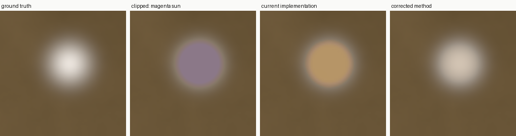
El caso desesperado totalmente recortado: un sol brillante quemado más allá del punto blanco (por canal) de cada canal, sobre un cielo naranja. El sensor registra un disco plano que los coeficientes RGB de balance de blancos volverán magenta; el método anterior devuelve un disco amarillo tenue y sobredimensionado con un borde duro (sus rellenos por canal se desvían de tono y nunca abovedar); el método corregido reconstruye una cúpula neutra del tamaño correcto a partir de una única cúpula de luminancia compartida más crominancia difundida desde el borde.
Sobre el núcleo recortado, RMSE $0.87 \to 0.27$ y SSIM $0.61 \to 0.95$; la crominancia del relleno se mueve de magenta $(0.37, 0.27, 0.36)$ a un casi neutro $(0.39, 0.33, 0.28)$, esencialmente el $(0.36, 0.33, 0.31)$ de la verdad de referencia (el método anterior aterriza en un amarillo $(0.51, 0.34, 0.15)$).
Añadir grano
Como toque final, y solo allí donde la máscara está abierta, la reconstrucción recibe ruido poissoniano de amplitud proporcional al valor local ($\sigma_c = \texttt{noise_level}\cdot u_c$), plegado para ser estrictamente aclarante y compuesto mediante $\alpha$. El ruido de disparo de fotones depende de la señal, de modo que un parche perfectamente liso insertado en un fotograma de alto ISO parece de plástico; igualar el grano hace que la reparación desaparezca.2
El radio de reconstrucción
¿Qué anchura debería tener la ventana guiada más gruesa, el radio de reconstrucción $\rho$? Es la única perilla que intercambia alcance por localidad, y resulta que tiene una respuesta limpia.
El radio de un agujero es su profundidad, no su tamaño. Para un agujero $\Omega$, sea $d(x)$ la distancia desde un píxel recortado $x$ al píxel válido más cercano. La cantidad que importa es el punto más profundo,
$$R=\max_{x\in\Omega} d(x)=\max\big(\text{distance transform of }\Omega\big)$$
no el rectángulo delimitador. Un disco compacto y una raya diagonal larga y fina pueden compartir un rectángulo delimitador mientras tienen valores de $R$ completamente distintos: para la raya, $R$ es su semi-grosor, porque esa es la distancia que la guía debe alcanzar para tocar datos válidos. Dimensionar el radio a partir del rectángulo delimitador sobrepasaría enormemente en agujeros alargados o diagonales.
Por qué $\rho \approx R$ es óptimo. Dos errores compiten a medida que $\rho$ crece. Cobertura: una ventana de escala $\rho$ pone un peso $\sim e^{-d(x)^2/2\rho^2}$ sobre los datos válidos, que es despreciable hasta que $\rho \gtrsim d(x)$; por debajo de eso el ajuste queda indeterminado y el píxel queda efectivamente sin reconstruir. Localidad: una vez cubierta, la línea de color ajustada es un promedio-ventana de la verdadera que varía espacialmente, así que extrapolar desde muestras cada vez más lejanas añade un sesgo que crece con $\rho$. El error por píxel es por tanto
$$E(x;\rho)\approx \underbrace{C_1\,e^{-d(x)^2/2\rho^2}}_{\text{coverage}\ \downarrow}+\underbrace{C_2\,\rho}_{\text{locality}\ \uparrow}$$
cuyo mínimo se sitúa en $\rho^*(x)\approx d(x)$: la ventana más pequeña que alcanza datos válidos. Un único radio de región debe cubrir su píxel más profundo, así que $\rho=R$; la escalera de grueso-a-fino es entonces exactamente este óptimo por píxel hecho continuo: la escala más gruesa $R$ sirve al centro, cada escala más fina sirve a la cáscara a su propia profundidad.
Sobrepasar es gratis en calidad, pero no en precio. En el prototipo, barrer $\rho$ desde $0.4R$ hasta $3R$ deja planos tanto el RMSE promedio como el del núcleo profundo, en escenas correlacionadas y en escenas decorrelacionadas por igual. La razón es estructural: la escalera de grueso-a-fino sobrescribe cada valor grueso (sobre-suavizado) con la escala más fina que aún alcanza al píxel, así que el radio fija solo la cobertura, nunca el valor final de un píxel. El cómputo, en cambio, no es plano (crece tanto con el área rellenada como con el número de escalas), así que la razón calidad-por-coste cae monótonamente con $\rho$:
| $\rho/R$ | RMSE promedio | RMSE núcleo profundo | coste relativo | calidad / precio |
|---|---|---|---|---|
| 0.4 | 0.083 | 0.141 | 0.43 | 1.00 |
| 1.0 | 0.083 | 0.141 | 1.00 | 0.43 |
| 2.0 | 0.083 | 0.141 | 2.39 | 0.18 |
| 3.0 | 0.083 | 0.141 | 4.43 | 0.10 |
El estudio del radio de reconstrucción: error y coste frente a la escala de ajuste como fracción del radio de la región. RMSE = error cuadrático medio frente a la verdad de referencia, 0 es una reconstrucción perfecta.
El punto óptimo es por píxel, y la implementación lo entrega. Como la calidad es plana por encima de la profundidad y el coste no lo es, la mejor calidad/precio es la ventana más pequeña que aún cubre cada píxel, es decir $\rho(x)=d(x)$ por píxel, nunca un máximo global. La escalera C realizaba esto directamente: una tesela fusionada tomaba el mayor radio del grupo $R$ como su escala más gruesa (de modo que el píxel más profundo quedaba cubierto), y cada píxel se limitaba entonces a escalas no más gruesas que $\sim2\,d(x)$, de modo que un píxel poco profundo (un agujero pequeño, o el borde de uno grande) nunca pagaba por las escalas gruesas que solo el centro necesita. La transformada de distancia se calcula una vez para todo el fotograma y controla el radio por región. La única regla firme es la asimetría: nunca ir por debajo de la profundidad (la cobertura se colapsa), y nunca muy por encima de ella (puro cómputo desperdiciado). El método distribuido mantiene la conclusión en una forma más simple: una ventana de ajuste dimensionada al radio de la región, $\sigma = \operatorname{clip}(r/6,\, 8,\, 64)$ px, sin ningún límite por píxel pendiente de aplicar.
Implementación y optimizaciones
Existen dos implementaciones: la referencia NumPy publicada junto a este artículo, y el código de producción C / OpenCL que se distribuye en Ansel. Se comparan uno contra otro como parte del protocolo de validación, y solo divergen allí donde la velocidad lo exige.
El código de producción en C
El prototipo que acompaña a este artículo es la referencia: favorece la claridad y la precisión sobre la velocidad (resoluciones dispersas-directas de imagen completa, una escalera gaussiana fija, un paso de varianza separado, un ajuste de línea de color por par (canal, guía)). El código que realmente se distribuye en Ansel tiene que reconstruir un sol recortado dentro de un raw de 20+ Mpx mientras el usuario espera, así que diverge de la referencia en un puñado de formas deliberadas. Cada compromiso a continuación está ajustado para contenido correlacionado, el caso abrumadoramente común en las imágenes naturales, y acepta una pequeña pérdida en contenido sintético decorrelacionado, que es raro en la práctica. Cada desviación es reversible en el código fuente. Una nota sobre la historia: este trabajo de optimización se hizo sobre el C de la era-escalera, cuyo núcleo de reconstrucción el método distribuido reemplaza. La segmentación, el rellenado, el solucionador disperso y la maquinaria de estadísticas compartidas se trasladan literalmente; los elementos específicos de la escalera (la escalera de escalas por agujero, el límite de profundidad por píxel, la elección de guía restringida por par) sobreviven solo como principios, dentro de la única ventana de ajuste y del relleno de coeficientes del método distribuido.
Segmentar y reconstruir solo los vecindarios recortados, a resolución completa. La referencia se ejecuta sobre el fotograma entero. El código distribuido rellena por inundación la máscara recortada en regiones conexas, rellena cada una con su propio radio de reconstrucción ($1.25\times$ el radio, acotado entre $8$ y $256$ px — cuanto mayor sea el agujero, más lejos debe alcanzar para hallar datos válidos), fusiona regiones cuyas cajas rellenadas se solapan de modo que sus rellenos nunca se junten como una costura, y ejecuta el pipeline completo solo dentro de cada caja rellenada. Coste: ninguno — los píxeles intactos ya eran correctos. Ganancia: el trabajo escala con el área recortada, no con el sensor.
Un Cholesky disperso independiente cerró la brecha del solucionador. La referencia rellena el domo de magnitud con una resolución directa dispersa (
scipy.spsolve); un solucionador iterativo (gradiente conjugado sobre $\Delta^2$) se estanca en precisión simple a escala raw (su número de condición, el factor por el cual el sistema amplifica los errores de redondeo, crece como la cuarta potencia del tamaño de la región), y una factorización densa es $O(N^3)$, así que el C distribuyó primero un Cholesky denso (la factorización exacta estándar de un sistema simétrico en mitades triangulares, calculada una vez y reutilizada) sobre una rejilla engrosada a como máximo 2000 incógnitas. Al ser el domo de baja frecuencia, la resolución gruesa era exacta donde importaba — salvo en núcleos enormes completamente quemados, donde el engrosamiento mismo se convertía en el cuello de botella de precisión (el caso de prueba del sol magenta mejoró un 21 % en RMSE el día en que se levantó el tope). El C ahora lleva su propio Cholesky disperso simétrico-definido-positivo (SPD), una factorización $LL^T$ ascendente en doble precisión, ordenada por disección anidada geométrica: las incógnitas son puntos de una rejilla 2D, así que la bisección recursiva de coordenadas entrega la calidad reductora-de-relleno que normalmente requiere una implementación de grado-mínimo-aproximado (AMD), en unas pocas docenas de líneas y sin dependencia externa. La rejilla del domo es cuatro veces más fina (8 192 incógnitas, lo que satura de forma medible la ganancia de calidad), y la difusión de crominancia del núcleo todo-recortado factoriza una vez para sus tres lados derechos de canal cuando el núcleo es pequeño; el gradiente conjugado paralelo supera de forma medible a la factorización serial en los grandes, así que los conserva. Coste: ninguno neto (las resoluciones todo-recortado se aceleraron). Ganancia: la última divergencia sistemática C-vs-prototipo desaparecida, y con ella la precisión del núcleo enorme.Una escalera gaussiana por agujero dimensionada al radio de reconstrucción. La referencia usa una escalera de radio fijo ($40, 24, \dots, 2$ px). La escalera C optimizada dimensionaba la escala más gruesa de cada región al radio de reconstrucción de esa región y la reducía a la mitad por $2\times$ hasta $\sim2$ px. Esto merece su propio tratamiento: ver El radio de reconstrucción más abajo.
Estadísticas de ventana compartidas: una aceleración gratuita. El ajuste de línea de color necesita, por par de canales, las medias, varianzas y covarianza de ventana. Reunirlas por (canal, guía) cuesta doce desenfoques por escala; reunirlas por par de canales produce los ajustes de ambos canales a partir de los mismos dos desenfoques: seis desenfoques, y matemáticamente idénticos. Esto por sí solo redujo aproximadamente a la mitad el tiempo de ejecución.
Varianza restringida por par para la selección de guía: un coste pequeño y contenido. La referencia decide cuál de dos guías fiarse a partir de la varianza de ventana de un solo canal de cada guía, un paso separado de tres desenfoques por escala. La escalera C optimizada reutilizó la varianza restringida por par que ya calculaba para el ajuste y eliminó ese paso por completo (nueve desenfoques por escala reducidos a seis). Esto cambió solo qué guía gana, y solo allí donde las dos discrepan, es decir, contenido decorrelacionado. Coste: en una escena sintética completamente decorrelacionada, el RMSE de recorte único sube de $0.043$ a $0.047$ y el SSIM cae de $0.964$ a $0.960$; en escenas correlacionadas, y en recorte de dos o tres canales, está dentro del ruido. Ganancia: eliminado un tercio de los desenfoques restantes.
El auto-domo por canal y el regularizador de costuras están deshabilitados en el código distribuido. Ambos suavizan cada canal RGB de forma independiente. En una alta luz ámbar/naranja real y saturada (donde el $R^2$ de la línea de color cae por la no-linealidad del recorte y se malinterpreta como “decorrelacionado”) eso desvía el verde respecto del rojo y el azul y vuelve magenta la reconstrucción. La referencia los conserva: eliminan artefactos de contenido genuinamente decorrelacionado, que las escenas sintéticas ejercitan intensamente y las fotografías reales rara vez presentan (deshabilitarlos le cuesta a la referencia $\sim0.01$–$0.02$ de RMSE en la escena aleatoria, esencialmente nada en contenido correlacionado). La solución limpia es una versión acoplada-en-matiz (suavizar la luminancia y una crominancia compartida en lugar de tres canales independientes), y desde entonces se ha construido: en el pipeline de campo-de-coeficientes final el auto-domo regresa como el respaldo limitado-por-profundidad, acoplado-en-matiz exactamente de esta manera (un domo de luminancia biarmónico compartido multiplicado por una crominancia rellenada armónicamente), de modo que el respaldo no puede desviar el matiz por construcción. El regularizador de costuras se retira definitivamente — ese pipeline no tiene ya transferencias de estimador que alisar.
Dos componentes de la implementación C de 2021 que la traducción del prototipo había descartado silenciosamente fueron reincorporados a la referencia, como auténticos requisitos del método más que como compromisos de velocidad, de modo que ya no son diferencias: el laplaciano de 9 puntos invariante a la rotación (el operador que este artículo deriva; la referencia usaba la sencilla cruz de 5 puntos antes567) y los suelos de saturación (abajo). Ambos mejoran el caso más difícil y relevante (el núcleo completamente recortado de una escena correlacionada), reduciendo su RMSE de $0.065$ a $0.062$ y elevando el SSIM de $0.959$ a $0.964$, y son neutros en el resto.
En conjunto, sobre un sol recortado el número de desenfoques del filtro guiado baja de quince a seis por escala y la reconstrucción de vista previa cae de decenas de segundos a unos pocos. Las diferencias que quedan son de velocidad y arquitectura (segmentación, solucionadores densos, el radio por agujero, estadísticas compartidas), más la varianza de guía restringida por par y el refinamiento por canal deshabilitado descritos arriba; la matemática central de reconstrucción se comparte con la referencia.
Un compromiso medido más se cerró pronto: la reconstrucción es notablemente mejor ejecutada a resolución completa. El módulo de 2021 resolvía sobre una copia a cuarto de resolución por velocidad, pero ese submuestreo desenfoca la reconstrucción y, fusionada de vuelta contra el original nítido, es la fuente dominante de error de borde: ejecutar a resolución completa redujo el RMSE de frontera en cerca de un 30%, así que la reconstrucción trabaja a resolución completa. El submuestreo es un compromiso velocidad/calidad, no un almuerzo gratis.
La referencia en Python
El espejo NumPy (validate.py, fix_prototype.py) implementa cada etapa del algoritmo distribuido
en el mismo orden, y comparar su salida contra las exportaciones C es parte del
protocolo de validación. Unos pocos componentes son deliberadamente mejores en Python que en C, o el C
deliberadamente intercambia exactitud por velocidad:
- Resoluciones directas dispersas exactas. Los domos biarmónicos del prototipo y su resolución de
crominancia en forma-de-divergencia son factorizaciones
scipy.sparse, exactas hasta la precisión de máquina (su relleno de núcleo-conjunto Poisson-cribado, sin embargo, es una relajación Jacobi fija de 400 barridos — en esa etapa la factorización directa del C es la más exacta de las dos). El C ahora lleva su propio Cholesky disperso (ver Implementación y optimizaciones arriba) e iguala las resoluciones de domo y de crominancia de núcleo-pequeño del prototipo; lo que aún difiere es deliberado: la difusión de crominancia de los núcleos grandes todo-recortado ejecuta el gradiente conjugado paralelo (medido como más rápido que una factorización serial ahí, sin diferencia de calidad medible), el relleno de coeficientes permanece como el Jacobi de grueso-a-fino descrito arriba — con la pirámide adaptativa del C (paso base $\sigma/4$ acotado en 8 px, reducido a la mitad hasta un nivel más grueso $\le 8$ celdas, 100 barridos por nivel) frente a los siete niveles fijos de resolución completa del prototipo — y el relleno del prototipo es isótropo — el guiado adaptativo-a-varianza del transporte de coeficientes del C (paso 3) no tiene aún espejo en Python, así que la concordancia C-vs-prototipo se comprueba teniendo en mente la contribución del guiado. Beneficio de las resoluciones exactas del prototipo: son el árbitro cuando la salida C parece incorrecta. - Ventanas gaussianas por FFT vs. IIR recursivo. El prototipo calcula los momentos de ventana con convoluciones por transformada rápida de Fourier (FFT): exactas, deterministas. El C usa la gaussiana recursiva (respuesta-impulsional-infinita, IIR) cuyo coste es independiente de $\sigma$ — pero cuya implementación paralela no es determinista de ejecución a ejecución: el redondeo en las fronteras de bloque fluctúa en el último dígito flotante, lo cual es inofensivo en sí mismo pero sembró un memorable heisenbug (abajo).
- Entrada de la estimación del codo. El prototipo estima la caída a partir de la escena RGB verdadera a resolución completa; el C a partir del CFA cuádruple-agrupado a $\le 1.5$ Mpx. Coste medido: ninguno (la estimación ciega del C aún iguala el codo analítico hasta $10^{-3}$), mientras que la agrupación cuádruple es lo que hace posible siquiera la estimación del lado-CFA.
- Fotograma completo vs. por-región. El espejo procesa fotogramas enteros; el C reúne cada región recortada en un búfer rellenado y la reconstruye de forma independiente, lo que acota la memoria y permite que las regiones se paralelicen, a costa de una normalización por región.
- Refinamientos distribuidos que el espejo aún no ha alcanzado. Tres rondas C tardías no tienen contrapartida en Python todavía: la maquinaria de obstáculos (relajación proyectada por nivel, el pulido a resolución completa, y el suelo suave de reensamblaje — el espejo aún aplica el retirado $\max(u, c_0)$ duro en el reensamblaje), la anulación de banda del umbral de detección para los canales con-codo-activado (vale $5\times$ en la escena de caída, así que Py-vs-C es estructuralmente incomparable ahí), y la validez binaria estrictamente por-píxel del C (el espejo deriva su máscara mediante un voto por mayoría 5×5, una dilatación geométrica de $\sim 2$ px). Estas son las brechas de contenido conocidas tras las mayores divergencias por escena.
Después de reflejar cada etapa, el desacuerdo residual entre el código de producción C y la referencia Python (medido como la diferencia cuadrática media de sus imágenes de salida dentro de las zonas recortadas) es de $0.009$–$0.089$ a lo largo del banco. Su suelo es la única diferencia de entrada que no puede eliminarse — Python ajusta sobre la escena RGB verdadera, mientras que el C ajusta sobre la misma escena vista a través del mosaico del sensor y una interpolación bilineal (a unos $0.02$ de distancia dentro de la banda cercana-al-recorte) — y su techo es la lista de refinamientos-distribuidos de arriba, que domina en las escenas de caída y de oclusión. Lejos de esas dos escenas, las implementaciones concuerdan bien dentro del error que cualquiera de las dos comete frente a la verdad de referencia; en ellas, la maquinaria extra del C es precisamente lo que mide la divergencia.
Parámetros de usuario
Deliberadamente no hay casi nada que configurar: el algoritmo es autoconfigurable. Cada
cantidad de la que depende la reconstrucción o bien se deriva una vez y se congela, o bien se mide a partir de la
imagen misma en tiempo de ejecución — la escala de ajuste a partir del propio radio de reconstrucción de cada región, la
caída del sensor a partir de las propias líneas de color de la imagen, la confianza del ancla a partir de la calidad de ajuste medida,
el guiado del transporte a partir de la estructura de guía medida, el umbral de borde $k$ calibrado
una vez sobre el banco de verdad-de-referencia. Los controles iterations y diameter del modo de 2021 han
desaparecido de la interfaz de este modo: no queda convergencia ajustable por el usuario que malconfigurar,
ni forma de sacrificar calidad por accidente.
Lo que queda es una seguridad y dos cuestiones de gusto. El clipping threshold escala los umbrales de saturación
que definen la zona (ver el conmutador de visualización más abajo — casi nunca necesita
moverse); el noise level fija el grano reinyectado sobre la reconstrucción para que iguale la
textura de fotones circundante; y inpaint a flat color fija la atracción hacia un
color uniforme en los núcleos completamente recortados donde nada sobrevivió — una elección estilística sobre zonas que
no portan información alguna.
Advice
El umbral de recorte tiene un conmutador de visualización-de-máscara (el icono junto al deslizador). Cuando está activo, el módulo renderiza una superposición de falso color (píxeles válidos atenuados, píxeles recortados señalados) para que puedas ver exactamente sobre qué región $\Omega$ actuará la reconstrucción antes de comprometerte con ella. Casi nunca deberías necesitar mover el umbral mismo.
Problemas descubiertos
La limitación estructural del método es heredada y aceptada: un cielo azul quemado visto a través de hojas verdes se recupera verde, porque allí donde ningún canal sobrevive la reconstrucción solo puede propagar el color vecino — fue diseñado para los recortes inevitables alrededor de fuentes de luz y reflejos especulares, cuyos halos resplandecientes portan la información de la que se alimenta. Otras situaciones aún exigen proteger las luces en la captura y elevar la exposición en posproducción, lo que la relación señal-ruido de los sensores modernos permite cómodamente.
Dos salvedades medidas completan el cuadro honesto. En la escena de oclusión del banco, la segmentación de Darktable ajustada alcanza una puntuación de similitud estructural más alta que la transposición armónica (0.98 frente a 0.96) a pesar de valores un 15 % más lejos de la verdad: magnitud y estructura son errores distintos, y un relleno erróneo suave puede parecer más limpio que uno veraz. Y la paridad de dispositivo del pipeline flotante es a nivel-de-tolerancia, no a nivel-de-bit: tras centrar la acumulación de momentos (paso 3), la diferencia residual CPU-versus-GPU en la escena más profunda del banco está por debajo de $10^{-3}$ RMSE, acotada por reducciones paralelas de orden-no-determinista.
Resultados
El banco
Every number below comes from one protocol. Six synthetic scenes with known ground truth — RGB
specular balls, a magenta sun, correlated gradients (a luminance field times a smooth
chrominance, how natural images behave), independent random gradients (no colour-line at all,
the adversarial case), a PK1-like sky with an analytic sensor rolloff, and a sun crossed by an
occluder — are written as Bayer DNG files, developed by the actual production pipelines, and
the exports are scored against ground truth in white-balanced sensor RGB (a full 3×3
calibration matrix fitted on strictly-linear valid pixels maps every export back to sensor
space, so differently-matrixed pipelines land in the same units). Every Ansel result in this
section — both modes, every table, every figure — is produced by the shipped C
implementation through ansel-cli, not by the Python research prototype : the two
implementations deliberately drift (different solvers, resolutions and stage trade-offs, see
the C production code), by 0.009 to 0.089 RMSE inside the clipped
zones across this bench, so their numbers must never be mixed. The whole bench reproduces
from the annex. (The white-balance campaign of the
addendum later added two scenes — a white emitter over
textured amber behind occluders, and a blown gradient sky — and a chromaticity-share metric,
because the six scenes above all clip at equal levels and linear RMSE is nearly blind to the hue
failures users actually report ; the numbers in this section are unaffected, by construction and
by re-measurement.)
Las métricas del algoritmo distribuido a continuación se calculan solo dentro del área recortada. El RMSE es el error cuadrático medio frente a la verdad de referencia, en unidades de sensor normalizadas de modo que el nivel de recorte es 1: mide cuán lejos están, en promedio, los valores reconstruidos de los verdaderos. El SSIM es el índice de similitud estructural, una puntuación perceptual que compara medias locales, contrastes y correlaciones (1 significa visualmente idéntico). La energía de borde es nuestro detector de costuras: la energía del gradiente-de-crominancia dentro de la zona, relativa a un anillo justo fuera de ella, y su objetivo es la puntuación de la propia verdad de referencia, no cero, porque el contenido real tiene textura y una reconstrucción sobre-suavizada es tan errónea como una con costuras:
| caso | RMSE | SSIM | energía de borde (objetivo GT) |
|---|---|---|---|
| bolas RGB | 0.0351 | 0.995 | 0.41 (0.47) |
| sol magenta | 0.3276 | 0.952 | 0.31 (0.50) |
| correlated | 0.0398 | 0.973 | 1.15 (1.14) |
| random | 0.0453 | 0.965 | 0.85 (1.02) |
| pk1synth | 0.0053 | 1.000 | 0.64 (0.69) |
| PK1 (natural) | — | — | 0.49 |
| DSC00078 (natural) | — | — | 0.73 |
| IMG_3129 (natural) | — | — | 0.39 |
La reconstrucción distribuida frente a la verdad de referencia, dentro de las zonas recortadas. RMSE = error cuadrático medio, 0 es una reconstrucción perfecta; SSIM = similitud estructural, 1 es una reconstrucción perfecta; energía de borde = magnitud media del gradiente, mejor cuando COINCIDE con la puntuación de la propia verdad de referencia (un relleno sobre-suavizado es tan erróneo como uno con costuras). Las naturales no tienen verdad de referencia, así que solo se muestra su energía de borde.
Los cuatro métodos
Los dos modos de Darktable se describen con las otras soluciones simples en la sección del panorama; leídos a través del marco de este artículo, inpaint opposed es una línea de color con la pendiente fijada en uno (en espacio de raíz-cúbica) y una única intersección global — donde la transposición armónica ajusta tanto pendiente como intersección por ventana local y difunde esos coeficientes a lo largo de la zona, opposed confía en una relación fija en todas partes, que es por lo que es casi gratis y por lo que falla bajo iluminación mixta — y segmentation based mejora eso a una crominancia representativa por segmento, todavía plana allí donde nuestros campos difundidos varían suavemente.
Ambos métodos responden a la pregunta “de qué color debería ser esta área”; ninguno ajusta un modelo de cómo el canal perdido se relaciona con los supervivientes, que es lo que permite a nuestro método recuperar estructura y magnitud por píxel con una confianza medida. Las filas de abajo ponen cifras a esa diferencia, sobre las mismas escenas sintéticas y verdades de referencia que todo lo demás en esta sección.
Error cuadrático medio (más bajo es mejor) y similitud estructural (más alto es mejor), medidos
dentro de la zona recortada frente a la verdad de referencia, tras la calibración de exposición por imagen; cada
método exportado como TIFF lineal de 32 bits (Darktable 5.x anterior para las dos primeras columnas, Ansel
para las dos últimas), puntuado por el mismo validate.py que cualquier otra tabla de esta página. Dos
precauciones hacen que las columnas sean realmente comparables. Primera, los pipelines se neutralizan a la
misma línea base — interpolación cromática más reconstrucción de luces, nada más: el flujo de trabajo referido-a-la-escena
por defecto de ambas aplicaciones inserta silenciosamente un realce de exposición, un mezclador de canales de adaptación-cromática
y una curva de tono sigmoide alrededor de su reconstrucción, lo que corrompería la medición con
diferencias de renderizado, así que se fuerza a workflow=none (la exportación de Ansel ya es esa
línea base). Segunda, cada competidor ejecuta sus mejores parámetros por escena, hallados por un barrido en rejilla
sobre sus controles (umbral de recorte para opposed; candidateo, combinar, modo de reconstrucción y
fuerza para segmentation; iteraciones y relleno de color-plano para los guided laplacians),
mientras que la transposición armónica ejecuta sus valores por defecto de serie en todas partes. Reproducir con dt_compare.py
(la comparación) y tune_methods.py (el barrido) del repositorio de investigación:
| escena | Darktable opposed | Darktable segmentation | guided laplacians | transposición armónica |
|---|---|---|---|---|
balls (bolas especulares) | 0.242 / 0.814 | 0.233 / 0.831 | 0.334 / 0.744 | 0.035 / 0.995 |
magentasun (sol magenta) | 0.924 / 0.707 | 0.807 / 0.767 | 0.809 / 0.678 | 0.328 / 0.952 |
correlated (gradientes correlacionados) | 0.107 / 0.872 | 0.077 / 0.907 | 0.130 / 0.850 | 0.040 / 0.973 |
random (gradientes independientes) | 0.089 / 0.911 | 0.080 / 0.920 | 0.138 / 0.862 | 0.045 / 0.965 |
pk1synth (cielo tipo-PK1 (caída analítica)) | 0.130 / 0.985 | 0.130 / 0.985 | 0.108 / 0.993 | 0.0053 / 1.000 |
occluded (sol ocluido) | 0.099 / 0.982 | 0.086 / 0.980 | 0.171 / 0.930 | 0.069 / 0.987 |
Los cuatro métodos frente a la verdad de referencia, como RMSE / SSIM por celda: RMSE = 0 es una reconstrucción perfecta, SSIM = 1 es una reconstrucción perfecta. Pipelines igualados a interpolación cromática + luces solamente, cada competidor en sus mejores parámetros por escena, todo puntuado en RGB de sensor con balance de blancos dentro de las zonas recortadas. Negrita = mejor de la fila.
El patrón es coherente con los mecanismos. Incluso con los pipelines igualados y cada competidor en su mejor por escena, la transposición armónica lidera en RMSE en cada escena — por un 20 % allí donde la oclusión favorece las suposiciones del modo de segmentación, por un factor de 2 a 7 en los casos generales, por un factor de casi 50 en el cielo de caída (donde la anulación de banda de más abajo permite al modelo reconstruir la pendiente que el sensor comprimió): los modos de Darktable recuperan un color plausible pero no la magnitud (su pendiente unitaria fija no puede elevar un canal por encima de lo que proporciona el promedio opposed), y su crominancia por-segmento o global aplana la textura. El modo de segmentación sí se adelanta al opposed simple una vez que su paso de reconstrucción está realmente habilitado (el barrido halló reconstrucción + fuerza completa óptimo en la mitad de las escenas). La contrapartida visual de cada cifra, una escena por galería, las seis versiones a través de la misma transformación de pantalla:
balls — bolas especulares:

la captura recortada

Darktable, inpaint opposed
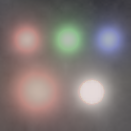
Darktable, segmentation based
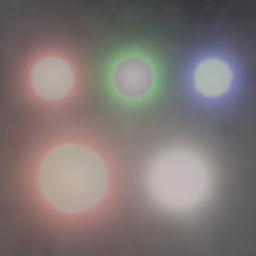
guided laplacians

transposición armónica

verdad de referencia
balls: cinco bolas especulares — rojo puro, verde, azul, un matiz mixto y blanco — cada una recortando una combinación de canales distinta; la prueba pura de recuperación-de-magnitud. Las seis versiones comparten una transformación de pantalla (normalizada al máximo de la verdad de referencia, gamma 1/2.2).
magentasun — sol magenta:

la captura recortada

Darktable, inpaint opposed

Darktable, segmentation based

guided laplacians

transposición armónica

verdad de referencia
magentasun: sol magenta — un disco completamente quemado sobre un gradiente de color, la prueba de estrés del núcleo-completamente-recortado. Las seis versiones comparten una transformación de pantalla (normalizada al máximo de la verdad de referencia, gamma 1/2.2).
correlated — gradientes correlacionados:
la captura recortada
Darktable, inpaint opposed
Darktable, segmentation based
guided laplacians
transposición armónica
verdad de referencia
correlated: gradientes correlacionados — un campo de luminancia por una crominancia suave, como se comportan las imágenes naturales. Las seis versiones comparten una transformación de pantalla (normalizada al máximo de la verdad de referencia, gamma 1/2.2).
random — gradientes independientes:
la captura recortada
Darktable, inpaint opposed
Darktable, segmentation based
guided laplacians
transposición armónica
verdad de referencia
random: gradientes independientes — sin línea de color alguna, el caso adversarial para los métodos basados-en-guía. Las seis versiones comparten una transformación de pantalla (normalizada al máximo de la verdad de referencia, gamma 1/2.2).
pk1synth — cielo tipo-PK1 (caída analítica):

la captura recortada

Darktable, inpaint opposed

Darktable, segmentation based

guided laplacians

transposición armónica

verdad de referencia
pk1synth: cielo tipo-PK1 con una caída de sensor analítica — la prueba de inversión-de-codo y anulación-de-banda. Las seis versiones comparten una transformación de pantalla (normalizada al máximo de la verdad de referencia, gamma 1/2.2).
occluded — sol ocluido:

la captura recortada

Darktable, inpaint opposed

Darktable, segmentation based
guided laplacians

transposición armónica

verdad de referencia
occluded: sol ocluido — un oclusor oscuro cruzando la zona quemada, la prueba de guiado-de-transporte. Las seis versiones comparten una transformación de pantalla (normalizada al máximo de la verdad de referencia, gamma 1/2.2).
El barrido completo del banco de validación (entrada recortada, reconstrucción, mapa de borde-de-crominancia ampliado, y verdad de referencia donde existe), más los perfiles de domo por canal, se muestra a continuación. Las gráficas de perfil se leen así: cada una toma la única fila de imagen que cruza el píxel recortado más profundo (recortada al tramo recortado de esa fila) y traza los valores de canal a lo largo de ella, un panel por canal, con la línea gris punteada en el nivel de recorte. Exponen exactamente lo que una miniatura oculta: la forma de la sección transversal del domo reconstruido, sus pendientes donde se encuentra con el borde válido, cuán por encima del nivel de recorte llega la recuperación, y cualquier sobreoscilación o zona plana — comparadas, en las escenas sintéticas, contra el propio perfil de la verdad de referencia. Todos los perfiles, imágenes naturales incluidas, se trazan en RGB de sensor con balance de blancos, por fotosito (los perfiles de imagen-natural leen el propio CFA, con el interpolación cromática puesto en modo passthrough) — el propio plano de trabajo del módulo, donde el invariante del suelo-de-saturación (un canal recortado nunca termina por debajo de su valor saturado) es directamente visible. Ninguna etapa posterior tiene esta propiedad: las diagonales-secundarias negativas de la matriz de color permiten que un canal reconstruido cruce legítimamente por debajo de su meseta de recorte (proyección de gama, no una violación de suelo), el interpolación cromática inventa dos de los tres canales en cada píxel y puede sub-oscilar en los bordes empinados de la reconstrucción, y cualquier remuestreador añade su propia sub-oscilación de Mitchell. Una característica de los perfiles naturales merece una advertencia: las estructuras oscuras que cruzan la zona quemada (aparejos, ramas, mástiles) son datos válidos medidos — la reconstrucción escribe solo fotositos recortados, así que el perfil se hunde a través de ellos en lugar de abovedarse sobre ellos. Una fila que cruza dos cuerdas retroiluminadas muestra dos lóbulos, y eso es la escena, no un fallo de reconstrucción:


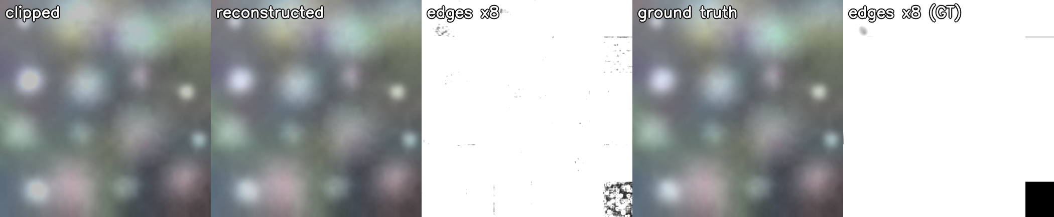



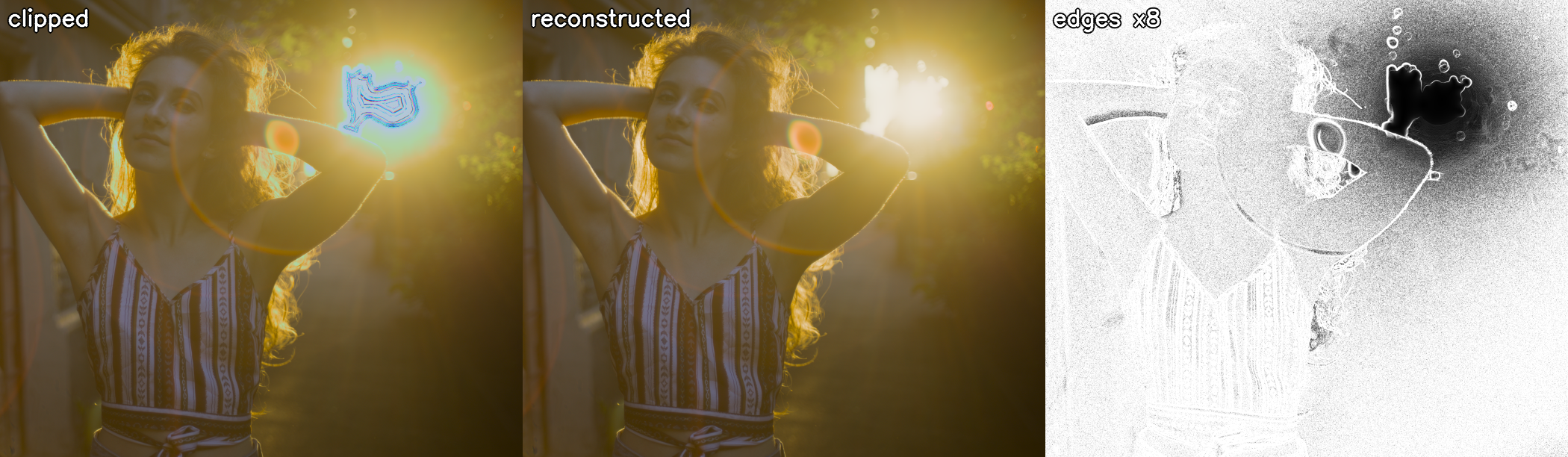

Rendimiento
Una reconstrucción que fuera mediblemente mejor pero inutilizablemente lenta no se distribuiría. Esta sección cierra
la historia con cifras: cómo escala el nuevo método, qué compró portarlo al procesador gráfico
(GPU, vía OpenCL), y cómo se comparan los métodos antiguo y nuevo en la misma máquina y las
mismas imágenes. El protocolo tras cada cifra a continuación es el mismo: cada medición de tiempo es una exportación completa
a través de ansel-cli, tomada como el mínimo de tiempo-de-reloj
de tres ejecuciones en una máquina por lo demás ociosa, con los tiempos internos del módulo leídos del
rastreo de rendimiento integrado.
Lineal en el área rellenada
Preguntar “qué tan rápida es la reconstrucción por megapíxel de imagen” es la pregunta equivocada: una imagen sin recorte cuesta casi nada, y el mismo sol quemado cuesta lo mismo tanto si el fotograma a su alrededor es de 12 como de 60 megapíxeles. La variable correcta se desprende de la estructura de costes. Cada etapa pesada del pipeline distribuido es lineal en el área de la región rellenada — la extensión de la zona recortada más el doble de su radio de reconstrucción, al cuadrado — con constantes independientes de la escala de ajuste: los momentos de ventana usan filtros gaussianos recursivos cuyo coste no depende del tamaño de la ventana, la difusión de coeficientes ejecuta un presupuesto fijo de cien barridos por nivel de pirámide sobre una rejilla base que se encoge a medida que crece la escala de ajuste (con la pirámide lo bastante profunda como para que su rejilla más gruesa sea trivialmente pequeña), y la resolución directa del domo de luminancia está acotada a un número constante de incógnitas (8192, sobre una rejilla diezmada) independientemente del agujero. Y como el radio de reconstrucción es el punto más profundo del agujero, el rellenado no es un parámetro libre: un agujero circular de radio $r$ necesita una región rellenada de aproximadamente $(4r)^2$ — dieciséis veces el propio rectángulo delimitador del agujero (la implementación rellena por $1.25\,r$ — el alcance mínimo más un margen de seguridad del $25\,\%$ — acotado entre $8$ px, para que las motas diminutas aún vean contexto, y un tope de coste de $256$ px, para que los agujeros más profundos crezcan algo más lento que esta ley). Duplicar el diámetro de una alta luz cuadruplica su coste, no porque el algoritmo sea superlineal, sino porque la reconstrucción honestamente necesita ver tanto más contexto.
El banco (make_perf_bench.py, reproducible) consiste en raws sintéticos con un único agujero circular
recortado de
radio creciente, en dos familias que ejercitan las dos rutas de código principales — un único canal recortado
(el campo de coeficientes hace el trabajo) y los tres canales recortados (lo hace el núcleo conjunto) —
cronometrados a través del pipeline de producción de línea-de-comandos, con cada región de las tres imágenes de prueba reales
superpuesta como puntos medidos. La máquina es un Intel Xeon E3-1505M v6, 4 núcleos / 8 hilos a
3.0 GHz.
| familia | radio del agujero (px) | región (Mpx) | campo de coeficientes + domo (ms) | núcleo conjunto (ms) | crominancia (ms) | total (ms) | ms / Mpx |
|---|---|---|---|---|---|---|---|
| canal-único | 56 | 0.10 | 135 | 0 | 1 | 136 | ~1360 |
| canal-único | 128 | 0.50 | 78 | 1 | 5 | 84 | ~170 |
| canal-único | 256 | 1.30 | 209 | 1 | 12 | 222 | ~170 |
| canal-único | 384 | 2.00 | 358 | 1 | 17 | 376 | ~190 |
| todo-recortado | 56 | 0.10 | 82 | 99 | 30 | 211 | ~2110 |
| todo-recortado | 128 | 0.50 | 137 | 90 | 221 | 448 | ~900 |
| todo-recortado | 256 | 1.30 | 384 | 222 | 1353 | 1959 | ~1510 |
| todo-recortado | 384 | 2.00 | 863 | 365 | 2375 | 3603 | ~1800 |
| PK1, cielo quemado (real) | — | 6.10 | 2689 | 4 | 60 | 2753 | ~450 |
| DSC00078, región más grande (real) | — | 2.80 | 1191 | 341 | 1943 | 3475 | ~1240 |
| IMG_3129, sol (real) | — | 0.50 | 660 | 44 | 35 | 739 | ~1480 |
Tiempo del módulo por etapa frente al área de la región rellenada (mejor de ejecuciones repetidas, ruta del procesador): dos familias sintéticas que acotan las rutas de código, más la región más grande de cada imagen de prueba real. La columna casi-constante ms / Mpx dentro de cada familia es la afirmación de linealidad.
Las cifras son mínimos por ejecución sobre ejecuciones repetidas del pipeline de producción completo. Leyéndola: por encima de aproximadamente medio megapíxel la ruta de canal-único mantiene 170–190 ms por megapíxel de región rellenada y la ruta todo-recortado 900–1800, a lo largo de una década de tamaños de región — la afirmación de linealidad, verificada; por debajo de eso, un suelo fijo por región de algún centenar de milisegundos (estadísticas de ventana en sus tamaños mínimos) domina y la lectura por-megapíxel pierde sentido. (La constante todo-recortado incluye el pulido de suelo-obstáculo de la crominancia del núcleo — ver el algoritmo — cuyo coste la puerta de actividad del pulido ahora exime allí donde el suelo de saturación no puede fijar; las correcciones de exactitud documentadas en los resultados compraron su calidad con trabajo honesto, y las rondas de optimización recuperaron lo que pudieron sin tocar la salida.) Dos ganancias estructurales llegaron desde la primera versión de esta sección. El solucionador directo disperso eliminó los cuellos de botella del domo y de la crominancia de núcleo-pequeño (la columna del núcleo-conjunto alcanza un pico de 0.3 s donde el Cholesky flotante denso gastaba segundos), y la resolución directa en forma-de-divergencia redujo la crominancia guiada-por-estructura a milisegundos allí donde el núcleo todo-recortado cabe en su tope de factorización. Y arreglar el umbral de semilla de la segmentación (hacía crecer regiones a través de residuo flotante de desenfoque-de-caja) encogió las regiones rellenadas mismas: el cielo quemado de PK1, antes un rectángulo rellenado de 15.8 Mpx, es ahora los honestos 6.1 Mpx — toda su reconstrucción tarda 1.3 s. Lo que domina ahora es la etapa del campo-de-coeficientes (momentos de ventana y rellenos armónicos, limitada-por-desenfoque) — que es exactamente donde el puerto OpenCL descrito abajo comienza.
Tiempo de reloj, antiguo versus nuevo
La comparación que los fotógrafos realmente sienten es el tiempo de exportación completa, modo antiguo contra nuevo, en la
misma máquina y los mismos archivos raw, bajo el protocolo enunciado arriba.
Tres casos naturales: PK1 (un archivo Bayer de 36 megapíxeles cuyo cielo quemado es una sola región de 6 megapíxeles
— el peor caso para el que se construyó el nuevo método), X-H1 (un archivo X-Trans de Fujifilm de 24 megapíxeles
cuyas luces se fragmentan en 99 regiones en su mayoría diminutas), DSC00078 (un atardecer Bayer de 24 megapíxeles),
y los dos extremos sintéticos del banco. Conviene recordar aquí que los guided laplacians se reducen de escala por un factor de 4, es decir un dieciseisavo de la resolución original, mientras que la transposición armónica se ejecuta a resolución completa. (Estos tiempos de reloj se remidieron tras toda la campaña de optimización de más abajo, en una sola sesión; la máquina llevaba un trabajo de fondo constante de un núcleo, que los mínimos por-celda sobre tres ejecuciones absorben en su mayoría.)
| exportación completa, tiempo de reloj | guided laplacians, procesador | transposición armónica, procesador | guided laplacians, tarjeta gráfica | transposición armónica, tarjeta gráfica |
|---|---|---|---|---|
PK1 (Bayer, un gran borrón) | 14.3 s | 11.4 s | 10.4 s | 9.8 s |
X-H1 (X-Trans, 99 regiones) | 9.3 s | 11.5 s | 6.9 s | 9.4 s |
DSC00078 (atardecer Bayer) | 16.6 s | 14.4 s | 11.4 s | 12.5 s |
occluded (sintética pequeña) | 0.9 s | 0.9 s | 1.2 s | 1.3 s |
allclip-384 (disco grande completamente recortado) | 2.2 s | 5.5 s | 1.9 s | 3.3 s |
Tiempo de reloj de exportación completa, modo antiguo contra nuevo, ambos medidos en una sola sesión (mejor de tres ejecuciones cada uno). Recuerda la asimetría: los guided laplacians reconstruyen a 1/16 de resolución, la transposición armónica a resolución completa, y sus tiempos de reloj incluyen la etapa de caída-del-sensor que el modo antiguo no tiene.
El titular honesto es que las ganancias de calidad documentadas en la sección de validación ahora vienen a un tiempo de reloj comparable o mejor casi en todas partes — el nuevo método gana la columna del procesador rotundamente en los archivos naturales, y solo el disco completamente recortado aún paga un sobreprecio real — y el camino hacia esa frase es instructivo, porque la primera compilación de producción del transporte anisótropo corría al doble de estas cifras allí donde las luces se fragmentan. Perfilar el archivo X-Trans de 99 regiones mostró que el coste no era aritmético: la relajación lanzaba un nuevo equipo de hilos por cada barrido (decenas de miles de lanzamientos de trabajo-de-microsegundo por imagen), los pesos de guiado se recalculaban en cada barrido aunque el tensor es fijo por nivel, y cada plano de coeficientes ejecutaba su propio relleno — su propia pirámide de máscara, su propio tensor — aunque los planos comparten ambos. Una región paralela por relajación, pesos precalculados una vez por nivel, y los planos de máscara-compartida fusionados en un solo relleno llevaron el tiempo de reloj del procesador de ese archivo de 18.3 s a 9.8 s — el guiado anisótropo en sí es esencialmente gratis en el procesador. Las correcciones de sesgo-de-borde y suelo-obstáculo documentadas en los resultados reinvirtieron entonces parte de esa ganancia en trabajo honesto (la validez binaria agranda los agujeros verdaderos; el pulido de obstáculo barre cada núcleo todo-recortado), y una ronda posterior recuperó parte de ella (los desenfoques de momento empaquetados de cuatro-en-ancho, el pulido condicionado a si su suelo puede fijar en absoluto), aterrizando en los 11.5 s de la tabla. Lo que queda es estructural. En el procesador el nuevo método gana allí donde su diseño rinde — en el caso del gran-borrón su trabajo es proporcional al área recortada (cada región resuelta una vez, exactamente) donde el método antiguo itera una difusión en cada escala de pirámide de la imagen entera — y sus tiempos de reloj aún incluyen una etapa que el método antiguo simplemente no tiene: la medición e inversión de la caída-del-sensor (0.7 a 1.2 s por sí sola en estos archivos) — con ella, el nuevo método ahora gana la columna del procesador en los tres archivos naturales. En la tarjeta gráfica el método antiguo mantiene una ventaja en escenas fragmentadas: un gran kernel uniforme por escala es la forma que los procesadores gráficos adoran, mientras que la cadena del nuevo método de etapas de solucionador pequeñas y mutuamente dependientes paga un coste de despacho fijo por paso. Dos respuestas medidas estrecharon esa brecha de inutilizable (el primer puerto ejecutaba el archivo de 99 regiones al doble del modo antiguo) a cerca de un 35 % sobre él: las regiones por debajo de un megapíxel saltan al procesador a través de una única transferencia empaquetada, y la factorización dispersa lanza un hilo por entrada de matriz en lugar de un grupo-de-trabajo por columna — ambas se cuentan en la sección OpenCL, y en el archivo de un-gran-borrón el nuevo método ahora también vence al antiguo en la tarjeta gráfica. Y el disco completamente recortado es el compromiso más claro de todos: sin canal superviviente en ninguna parte no hay línea de color que ajustar, y las resoluciones exactas de domo y matiz del nuevo método compran su calidad — sin relleno plano, sin deriva de matiz, sin borde visible — a cerca de 2.5 veces el precio de la difusión antigua en el procesador (1.7 en la tarjeta gráfica), precisamente en el caso donde la salida del método antiguo está en su punto más débil.
El pipe OpenCL
El primer puerto OpenCL era híbrido: la interpolación y el remosaico final se ejecutaban como kernels de dispositivo, pero la parte media de la reconstrucción se ejecutaba en el procesador, sobre planos descargados de la tarjeta gráfica y resubidos después. Ese diseño era neutral-en-coste — las transferencias se comían lo que los kernels ahorraban — y fue rechazado exactamente por esa razón: dar dos idas y vueltas a una imagen de 36 megapíxeles por el bus dos veces por exportación es la clase de impuesto que silenciosamente domina un pipeline.
El puerto distribuido tiene cada etapa de la reconstrucción en el dispositivo — la interpolación, los rellenos de coeficientes, las pirámides anisótropas, los solucionadores dispersos, el remosaico (una excepción: pedir regeneración de grano enruta la reconstrucción a través de la ruta del procesador). Pero tener cada etapa en el dispositivo no es lo mismo que ejecutar cada región allí, y el diseño final no lo hace. Instrumentar el tráfico anfitrión–dispositivo del puerto (contadores de sincronización en cada lectura bloqueante, drenaje de cola y lanzamiento de kernel, impresos con el rastreo de rendimiento) contó una historia que los tiempos de etapa del perfilador habían ocultado: las lecturas-de-vuelta bloqueantes que todos culpan primero cuestan un despreciable ~150 ms por exportación, mientras que el conteo de lanzamientos era el impuesto — cerca de mil lanzamientos de kernel por región, independientemente del tamaño de la región, porque las etapas iterativas lanzan por barrido y las resoluciones dispersas lanzan por nivel de árbol-de-eliminación. Una región de 700 píxeles midió 22 ms en el dispositivo frente a menos de 1 ms en el procesador: todo despacho, nada de aritmética. En el archivo de prueba X-Trans — 99 regiones en su mayoría diminutas — eso eran más de 100 000 lanzamientos por exportación, con el tiempo de reloj ejecutándose al doble del tiempo ocupado del dispositivo.
Así que el pipe distribuido enruta cada región al lado del bus que midió más rápido. Las regiones de hasta cerca de un megapíxel son empaquetadas por un kernel en un búfer de preparación contiguo, cruzan el bus en una sola lectura-de-vuelta, son reconstruidas por la ruta de producción del procesador sobre la ventana trasladada, y regresan a través de una subida y un kernel de dispersión-espejo — dos lanzamientos y dos transferencias en lugar de mil lanzamientos. Este no es el híbrido rechazado del primer puerto volviendo por la ventana: aquel daba una ida y vuelta a la imagen entera por exportación, un coste proporcional al sensor; este mueve solo los vecindarios recortados, un coste proporcional al daño — la ventana de dos-transferencias para una región pequeña es miles de veces menor que una ida y vuelta de fotograma-completo. Las regiones grandes — un cielo quemado de seis megapíxeles — permanecen totalmente residentes en el dispositivo, donde el masivo paralelismo uniforme gana genuinamente.
La ruta de región-grande residente-en-dispositivo obtuvo su propia corrección medida. La factorización Cholesky dispersa se ejecuta nivel-por-nivel sobre su árbol de eliminación (las columnas que no dependen unas de otras se procesan juntas), en flotantes de 64 bits en el dispositivo — pero el primer puerto daba a cada columna un pequeño grupo-de-trabajo, y cerca de la raíz del árbol un nivel contiene un puñado de columnas: el dispositivo permanecía ~98 % ocioso durante cientos de niveles, y la región grande del archivo de atardecer pasaba dos segundos factorizando. El kernel distribuido en cambio agrupa, en el momento del análisis-simbólico, cada contribución de actualización por la entrada de matriz en la que aterriza, y lanza un hilo por entrada de matriz por nivel — sin atómicos, sin barreras, y las contribuciones se acumulan en el orden exacto que el código secuencial usaba, así que la factorización es reproducible-a-bit: la mayor diferencia procesador-versus-dispositivo de la autoprueba no se movió ($10^{-12}$, relativa). El mismo agrupamiento simbólico hizo paralelo el análisis del lado-anfitrión, reduciéndolo a la mitad también. Los sistemas sobredimensionados aún recurren a los mismos esquemas de gradiente-conjugado y grueso-a-fino que la ruta del procesador. El relleno de coeficientes guiado es residente-en-dispositivo también: el plano de guiado, sus tensores de estructura por-nivel, los pesos de borde precalculados y la relajación ponderada de ocho-vecinos se ejecutan todos como kernels, e incluso la reducción de gradiente-medio de la normalización del tensor se termina en el dispositivo — nada cruza el bus a mitad-de-relleno (una versión anterior leía la reducción de vuelta por nivel, y cada lectura-de-vuelta drenaba silenciosamente toda la cola de comandos).
Lo que cruza el bus, entonces: máscaras de un-byte-por-píxel (para la segmentación, cuyo análisis de componentes-conexos permanece en el procesador), un plano de profundidad, los planos de momento cuádruple-agrupados del estimador de codo (a lo sumo un par de megapíxeles de flotantes), unos pocos kilobytes de resultados de reducción, y las ventanas de región-pequeña recién descritas. Cada etapa se valida contra su gemela del procesador mediante una autoprueba que ejecuta ambas sobre la misma escena sintética e imprime la mayor diferencia — entre $10^{-5}$ y $10^{-12}$ según la etapa. En cinco de las seis escenas sintéticas, las exportaciones de imagen-completa en dispositivo igualan la salida del procesador dentro de un 0.31 % de la escala completa en el peor píxel, con cero píxeles por encima del 1 %; la escena de oclusión es la excepción honesta — las interpolaciones del dispositivo y del procesador discrepan en una muestra en el borde de contacto del oclusor y la reconstrucción la amplifica ahí, así que 22 píxeles (de 786 000) superan el 1 %, alcanzando el peor un 10 %. Es una diferencia de recolección conocida, localizada y preexistente, no una del solucionador.
Dos lecciones de ese puerto se generalizan. Primera, el procesador gráfico no es más rápido en todo, y la respuesta honesta es medir y enrutar: esta carga de trabajo es una larga cadena de pasos pequeños y mutuamente dependientes — solucionadores iterativos, niveles de pirámide, bucles por-región — y un dispositivo paga un coste de despacho fijo por paso. El agrupamiento ayuda enormemente (cien iteraciones de suavizado en un solo lanzamiento; los planos de coeficientes que comparten una máscara avanzando juntos en cada lanzamiento; un hilo por entrada de matriz en lugar de un grupo-de-trabajo por columna), pero por debajo de cierto tamaño de región ninguna cantidad de agrupamiento vence a un procesador cuyo coste de despacho es una llamada de función — así que por debajo de ese tamaño, medido en cerca de un megapíxel, el pipe simplemente usa el procesador. Segunda, la ganancia es sistémica, no local: con el pipeline residente en el dispositivo de extremo a extremo, los módulos circundantes nunca se estancan y nunca transfieren, y lo que el módulo de luces devuelve por el bus ya no es la imagen — es solo el daño.
Hallazgos teóricos
Más allá del software distribuido, la campaña produjo resultados que no son específicos de la reconstrucción de luces — ni siquiera de la fotografía. Esta sección reúne tres resultados generales sobre trasladar modelos a través de vacíos de datos y coser estimadores juntos; un cuarto resultado reutilizable, la ley de escala de cuán lejos debería alcanzar una reconstrucción, se deriva con el método que dimensiona en la discusión del algoritmo.
Las tres lecciones más trascendentes de la campaña se citan en el resumen y se dispersan por las secciones de arriba, pero merecen un enunciado propio, porque nada en ellas es específico de la reconstrucción de luces: la primera es un método para trasladar una relación medida a través de un vacío de datos, y las otras dos deberían valer para cualquier problema donde varios estimadores de la misma señal desconocida deben coexistir en una imagen.
Transporta el modelo, no los valores. La reconstrucción distribuida cruza la zona quemada difundiendo los parámetros de un modelo local — los coeficientes de la línea de color — en lugar de la señal misma. Eso suena engañosamente cercano a algo que el filtro guiado siempre ha hecho: el filtro original de He, tras ajustar su modelo afín en cada ventana, desenfoca los coeficientes ajustados antes de aplicarlos, y una media local es un desenfoque, que es un paso de difusión. La distancia entre ese paso y este método merece explicitarse, porque es donde pivota todo el diseño.
He promedia ajustes que existen; nosotros construimos ajustes donde ninguno puede existir. En el mundo del filtro guiado, cada píxel está observado: cada ventana produce un ajuste válido, cada píxel se sitúa dentro de muchas ventanas solapadas, y el desenfoque simplemente arbitra entre sus respuestas en competencia. En lo profundo de un agujero recortado, una ventana no contiene ninguna muestra válida del canal que se reconstruye: no hay nada que ajustar, por tanto nada que promediar. Un desenfoque lleva información a lo sumo un radio de kernel; más allá de esa profundidad, un plano de coeficientes desenfocado sigue estando vacío.
Un solo paso de suavizado versus el límite de infinitos. Una media local aplicada una vez tiene un rango fijo. Nuestro relleno repite la misma operación — reemplazar cada incógnita por la media de sus vecinos — hasta la convergencia, con los ajustes de confianza fijados. El límite ya no es un desenfoque: es la solución exacta de un problema de valores-en-la-frontera (la ecuación de Laplace, con los anclajes como frontera), no tiene escala incorporada, cruza un agujero de quinientos píxeles tan fácilmente como uno de cinco píxeles, y pondera cada anclaje por la geometría real del agujero en lugar de por un kernel fijo. Itera la media de coeficientes de He para siempre con los ajustes válidos fijados y obtienes exactamente este relleno. He se detiene en un solo paso porque su problema solo necesita un arbitraje suave; el nuestro debe llevar el modelo a través de cientos de píxeles de nada. La diferencia de grado se convierte en una diferencia de tipo: la regularización se convierte en extrapolación.
Una media toma a todos; una frontera toma solo a los testigos. La media de He incluye cada ajuste de ventana, también los degenerados — parte de por qué su fórmula necesita su constante estabilizadora. Aquí, un ajuste se convierte en anclaje solo si puede responder por sí mismo: suficientes muestras de confianza en su ventana, una calidad de ajuste por encima del umbral, pendientes acotadas. Los malos ajustes se excluyen de la frontera en lugar de diluirse en ella, y el principio del máximo entonces garantiza que los coeficientes rellenados nunca abandonan el rango de los buenos. La calidad de ajuste se difunde ella misma junto al modelo, como un plano más, así que cada etapa posterior sabe cuánto merece ser confiado el modelo transportado en cada píxel.
El papel se invierte: de corrección a portador. En el filtro guiado, el suavizado de coeficientes es una pequeña corrección encima de datos que existen en todas partes. Aquí, el campo difundido es el único portador de la reconstrucción a través del agujero, y los datos reingresan al final: el modelo transportado se evalúa contra los canales supervivientes medidos en cada píxel. Un campo suave aplicado a datos medidos nítidos da un resultado nítido. El modelo aporta la relación; los datos aportan el detalle.
Enunciado sin fotografía alguna: cuando una señal tiene vacíos, pero un modelo de ella ajustado localmente varía suavemente, entonces ajusta el modelo allí donde los datos lo sustenten, conserva solo los ajustes que puedan responder por sí mismos, rellena los parámetros del modelo a través del vacío mediante una difusión de estado-estable anclada (una resolución de valores-en-la-frontera, no un desenfoque), lleva la confianza del ajuste a lo largo como un campo más, y reevalúa el modelo transportado contra cualesquiera datos que sobrevivieran dentro del vacío. Los valores lejos de los datos son inestables; los modelos lejos de los datos son simplemente suaves.
Esa extensión se ha construido, medido y distribuido desde entonces: el relleno ahora se guía anisótropamente por la estructura de los canales supervivientes (paso 3 tiene la matemática). A diferencia de la cuestión indecidible de si la línea de color se cumple donde nada se mide, las guías sí se miden dentro de la zona parcialmente-recortada, así que el guiado se ejecuta sobre evidencia, no sobre conjeturas. El experimento enseñó dos lecciones dignas de registrarse. Primera, la mayor “ganancia” del primer prototipo resultó ser un artefacto de convergencia: los cien barridos de relajación fijos por nivel de pirámide truncaban el relleno isótropo simple en agujeros profundos, y simplemente convergerlo recuperó la mayor parte de la mejora (22 % del RMSE en el cielo sintético más profundo) — detectado solo porque el control isótropo se reejecutó con recuentos de barrido igualados, una pequeña victoria más del banco sobre la historia plausible. Segunda, a igual convergencia los dos guiados puros dividen las escenas exactamente como la teoría predice: el transporte radial gana en todas partes donde el halo está limpio, el transporte a-lo-largo-de-la-frontera gana solo donde un borde cruza la zona, y ninguno domina. El tensor distribuido por tanto los mezcla por celda, ponderando por una varianza de ventana corregida-en-tendencia que separa “rampa empinada pero suave” de “borde duro” — y con ello el relleno nunca es peor que el isótropo en ninguna escena de verdad-de-referencia, y mejor por un 7 % (cielo profundo) a un 2 % (oclusión) allí donde el guiado tiene algo sobre lo que actuar.
La ley de energía-de-costura. Siempre que dos estimadores $A(x)$ y $B(x)$ de la misma señal se mezclan sobre una zona de transición por un peso $w(x)$ (una máscara dura, una máscara difuminada, o una confianza por-píxel, no importa), el compuesto es $u = w\,A + (1-w)\,B$, y su gradiente se divide en tres términos:
Los dos primeros términos son la estructura propia de los estimadores, que aparece y desaparece gradualmente. El tercero es la costura: existe solo donde el peso varía (la zona de transición), y su intensidad es el desacuerdo $A-B$ de los estimadores allí, multiplicado por la rapidez con que viaja el peso. Dicho llanamente: pasar de un estimador a otro imprime un borde cuyo contraste es exactamente cuánto discrepan los dos en el cruce. Y el peso no puede negociar su salida: aún debe subir de 0 a 1, así que una rampa más abrupta concentra la costura en una línea mientras que un difuminado más ancho la diluye en una banda poco profunda — la energía total de la costura la fija el desacuerdo por sí solo. Por eso los siete esquemas de ponderación de el cementerio fallaron de forma idéntica: eran siete formas de $w$ frente a un invariante. Las dos únicas salidas son las que el algoritmo entregado toma en todas partes: hacer que los estimadores concuerden en la transición (la inversión de la rodilla desvía los datos para que la extrapolación y la medición se encuentren en el contorno de detección), o eliminar la transición (un único estimador, prolongado suavemente por toda la zona: los campos de coeficientes).
La indecidibilidad de la línea de color. La hipótesis central de la reconstrucción es que la proporcionalidad local entre canales (la línea de color) medida en el borde válido se mantiene aún en lo profundo de la zona quemada. Aquí está el porqué ningún algoritmo puede verificar esa hipótesis a partir de la imagen: construye dos escenas idénticas píxel a píxel en cada valor medido, pero que difieren dentro de la zona quemada — en una de ellas la alta luz oculta un objeto cuyo color rompe la línea; en la otra no. Ambas escenas producen la misma entrada, y sin embargo exigen reconstrucciones distintas; cualquier estimador, por astuto que sea, responde de forma idéntica para ambas y por tanto se equivoca al menos en una. La escena sintética ocluida del banco es exactamente esta construcción, y se comportó como el argumento predice: las cinco compuertas candidatas medidas en el cementerio — calidad del ajuste, validación del borde, coherencia de la pendiente y las demás — no lograron detectar a partir del entorno si la línea se mantenía en el interior. La consecuencia práctica dio forma al diseño entregado: puesto que la pregunta no puede decidirse, debe cubrirse — la fusión con compuerta por profundidad se inclina progresivamente de la línea de color hacia la cúpula de luminancia suave a medida que crece la distancia a cualquier dato medido, no porque se sepa que la línea falla allí, sino porque nada puede dar fe de ella.
Addendum : the white-balance clip regime
(Added 2026-08, after field testing on real raws.)
The bench above declared victory, and users kept reporting magenta. Both were right. Every synthetic
scene in the bench writes AsShotNeutral = (1,1,1), so the production pipeline develops it at unit
white balance — all three channels clip at the same level. No real camera occupies that regime : the
module runs after the temperature stage, so on a real raw the per-channel clip levels are the
white-balance gains, typically $(2.3, 1.0, 1.3)$ and beyond. Everything in this addendum follows from
taking that regime seriously : two new failure families were isolated on real photographs, measured to
their root causes, and fixed behind gates that leave every number in the article above bit-for-bit
untouched. The campaign also extended the bench so the regime stays covered.
The floors author the colour
The lead complaint (clipped neon tubes rendered magenta) survived three plausible theories — an X-Trans phase mismatch, demosaic bleed, a fit-slope error — each killed by measurement before the real mechanism surfaced, and it is embarrassingly close to the one this article opened with. Dumping the module’s own output and bucketing per-channel means by “own channel clipped” against the per-channel clip levels showed the clipped channels sitting exactly at their floors. The saturation floor is per-channel : on a multi-clip pixel whose extrapolation undershoots, each clipped channel snaps to its own level, and the ratio between the floors — the white-balance gains, i.e. magenta — replaces whatever hue the solver produced. The solver’s chroma was fine ; the floors destroyed it. (The 2021 method looked whiter on the same subjects only because it violates the floors — dimmer, not less wrong.)
The fix preserves the floors’ physical guarantee while removing their colour authority : a joint floor lifts the whole clipped subset by one scalar $s = \max_k(t_k / e_k)$ until the most demanding per-channel target is met — brightness from the floors, hue from the solver — identical to the per-channel floor wherever a single channel clips, capped at 8× with the per-channel floor kept afterwards as the degenerate-estimate safety net.
Applied unconditionally, this regressed the whole bench : at equal clip levels the per-channel
imprint is neutral, usually near the truth of a bright core, and materially helpful. The regime is
detectable from the clip levels alone, so the joint floor is blended in by a clip-asymmetry gate
$g = S\big((A - 1.25)/0.75\big)$ with $A = \max_c \text{clip}_c / \min_c \text{clip}_c$ : zero
through the whole unit-white-balance regime, one from $A \ge 2$, which every real camera reaches. Two
traps are worth recording. The ramp must not start at $A = 1$ : the clip levels inherit the
pipeline’s input profile handling, which carries a ~10 % non-white-balance wiggle even on the
unit-balance DNGs (measured $A = 1.145$ on this very bench) — a ramp from 1 silently opened the gate
to 0.2 on the regression suite and contaminated a whole candidate round before it was caught. And the
synthetic DNGs cannot exercise the gate through the production pipeline at all : temperature
ignores their AsShotNeutral, so the C-side regression guard is bit-identity at gate zero, and the
regime itself is validated on real raws and through the Python leg described below.
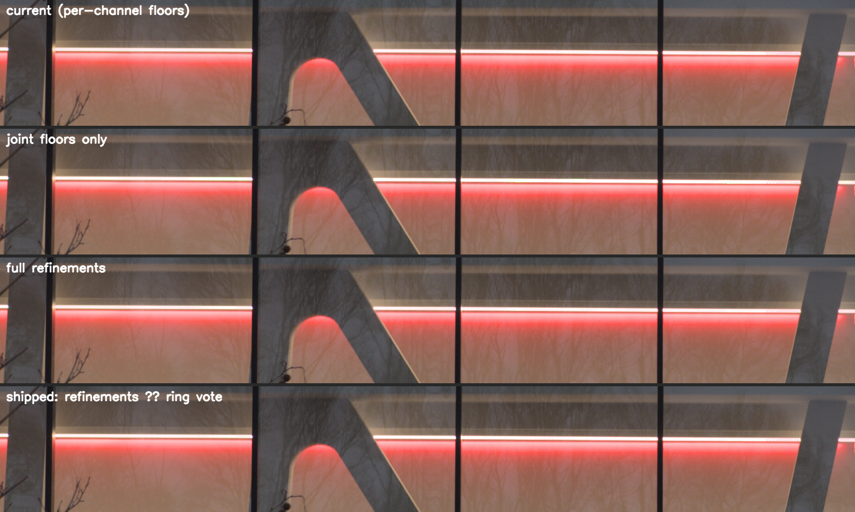
The clipped neon tubes, four ways. Top to bottom : the article’s method as published (per-channel floors — the tubes and their glow drift magenta) ; the joint floor alone (hue restored where the solver spoke, about two thirds of the visible fix) ; the surround refinements added (the shipped look) ; the shipped configuration with the trusted-ring vote arbitrating the refinements.
Continuing the surround : chromaticity gradients and their gate
The second family (blotchy pink-lavender patches and occluder-shaped chroma ghosting inside a blown sunrise) traced to a bias every value-continuing estimator in the method shares : colour-line fits and harmonic ratio fills anchor on the last unclipped band before the clip contour, and that band is not the scene — it is sensor rolloff and veiling flare, whitened and threaded with occluder penumbras. Hardening the dim-anchor rejection made it worse (it starved the windows ; the dark anchors were warm, not the contaminant), and shrinking slopes toward a mean-ratio prior plateaued short because the prior inherits the same fence hue.
The shipped stage extends the bright, fully-valid surround’s chromaticity shares into the blown zone with the same biharmonic, gradient-continuing operator the luminance dome already uses, then reprojects each partial multi-clip pixel’s clipped subset onto the extended field — the surviving channels anchor the brightness, the clipped ones take the field’s shares. Three hard-won details : the anchors stand clear of a thin guard ring around the contour (a wide moat exiles them to unrepresentative far content and inverts the fix) ; all-clip pixels are not reprojected (redistributing a poor core total by the field’s shares was measured to produce negative pixels) ; and the whole continuation is a scene assumption, true for gradient skies and false for self-coloured emitters, so it arbitrates itself against the method’s trusted zone : at 1-clip pixels — rebuilt from two measured guides — the field either agrees with the solver or it does not, and the agreement weight, diffused inward with a region-level ring vote as fallback, gates the reprojection. On the white-lamp complaint above the gate correctly reads the lamps as self-coloured and stands down — which is how it was established that the magenta fix could not come from this stage and had to come from the floors.
The surround refinements and the trusted-ring vote
Between the floors and the continuation sit three smaller surround-importing refinements, all gated by the same clip asymmetry : the self-dome’s filled chroma is pulled toward the bright surround mean, multi-clip pixels are re-projected onto the dome’s chromaticity instead of blending per channel, and the all-clip core’s floor is re-hued (magnitude-preserving) toward the surround mean so the downstream stages stop treating the inverse-gain magenta as a colour target. They fix the last third of the neon complaint and land the sunrise on the warm side — and they are exactly as dangerous as they sound : on a genuinely self-coloured emitter they paint the surround over the subject. Their arbitration took three measured failures to get right (all in the graveyard) : a per-pixel agreement average is capped near 0.3 on any real ring by noise and texture spread, at every tolerance tight enough to still protect the emitter ; referencing the whole-window valid mean lets dark unrelated content close the gate on exactly the scenes the refinements serve ; and a bright-surround dispersion factor turned out inverted on the one scene it was designed for. What separates the regimes is not how much the trusted ring disagrees but how coherently : a self-coloured emitter shifts its whole 1-clip ring to one side of the bright-surround mean, while real scenes scatter around it. The shipped vote is a t-statistic, $t = |\text{ring mean} - \text{surround mean}|_1 / \max(\text{ring dispersion}, 0.02)$ mapped through $e^{-(t/5)^2}$ — measured at $t \approx 10$ (vote ≈ 0) on the self-coloured bench emitter and $t = 0.3$–$1.5$ (vote ≈ 1) on the real photographs.

The self-coloured emitter that polices the refinements, in the white-balance regime leg (left to right : clipped input, per-channel floors, joint floors only, full refinements, refinements × ring vote, ground truth). Ungated refinements (fourth panel) paint the surround over the magenta sun and more than double its chroma error ; the ring vote (fifth panel) reads the coherent shift of the trusted ring and stands down, landing on the safe column."
Extending the bench to the regime
The bench gained two scenes — wbclips, a white emitter over textured amber behind mullion
occluders written with real white-balance metadata, and gradsky, the blown-gradient-sky geometry —
and a chromaticity-share RMSE (the per-pixel share error $u_c/\sum u$, ×100) reported alongside
linear RMSE, which is magnitude-dominated and nearly blind to hue. Because the production pipeline
ignores the synthetic white-balance metadata, the regime itself is exercised by a Python leg that
clips in the physically correct order : the ground-truth scene is clipped at the sensor, multiplied
by the gains, reconstructed in that domain, divided back, and scored. The shipped configuration
against that leg :
| case | per-channel floors | shipped |
|---|---|---|
| RGB balls | 0.040 / 0.27 | 0.055 / 0.35 |
| magenta sun | 0.354 / 1.29 | 0.354 / 1.30 |
| correlated | 0.027 / 0.49 | 0.030 / 0.62 |
| random | 0.044 / 1.00 | 0.044 / 1.01 |
| PK1-like sky | 0.115 / 2.95 | 0.113 / 2.90 |
| occluded sun | 0.096 / 2.47 | 0.088 / 2.36 |
white emitter / amber (wbclips) | 0.877 / 2.92 | 0.723 / 1.40 |
gradient sky (gradsky) | 3.450 / 3.55 | 3.442 / 0.95 |
The white-balance regime leg (sensor clip, then gains (2.2, 1.0, 1.5)), scored against ground truth inside the clipped zone : linear RMSE / chromaticity-share RMSE ×100. ‘Per-channel’ is the article’s published behavior in this regime ; ‘shipped’ is the gated joint floors, refinements × ring vote, and value continuation. The emitter row is the safety case : the vote must keep the shipped column at the per-channel column’s chroma.

The gradient-sky case in the white-balance regime (clipped input, per-channel floors, joint floors only, full refinements, shipped, ground truth) : the chromaticity-share error drops from 3.55 to 0.95 — the hue failure the original bench could not see, fixed by the machinery the original bench could not exercise."
The chroma error halves on the emitter-over-amber case and drops almost fourfold on the gradient
sky, while the self-coloured emitter is held at published behavior by the vote — the regime’s
victory condition. The small losses on balls and correlated are the price of the arbitration
and are invisible at the display ; the two real photographs that motivated the campaign were
accepted visually at every step.
Open in this regime
Two limits are measured and waiting. Veiling flare on measured data, described above : the reconstruction’s contract ends where measurement begins, and the flare lives in the measurements. And a window-scale blindness found on a blue LED lamp array : with a large blown region the fit windows clamp at $\sigma = 64$ px and cannot resolve the 5–20 px interstices between bulbs, while the soft-luminance affinity that normally separates unrelated content within a window is blind there, because the clipped-high channel dominates the luminance of bulbs and interstices alike — so anchored, high-confidence fits deliver bulb-level coefficients to glow-level pixels, and the display clips the over-lift to pale, mask-shaped fingers. Every localized patch tried against it (a contour feather, gated and ungated ; split anchor sets for the intercept transport) was measured useless or harmful and is recorded in the graveyard ; the honest candidates are a valid-channel-only luminance affinity, or multi-scale fit windows — both method-level changes, neither yet built.
Cómo se hizo realmente este trabajo
El método anterior es inseparable de la forma en que se produjo, y la forma en que se produjo partió de una confesión. Los guided laplacians de 2021 fueron el último método que entregué antes de escribir sus matemáticas: programado contra la intuición, ajustado a ojo sobre imágenes naturales. Eso alcanza un primer resultado rápidamente y es ciego a todo lo posterior — no puedes estudiar las propiedades ni los modos de fallo de un método que solo ejecutaste sobre datos no controlados. Escribir este artículo, para asentar por fin esas matemáticas, impuso la disciplina opuesta: escenas sintéticas con verdad de referencia (ground truth) conocida, métricas de error objetivas, una hipótesis probada a la vez. Esa disciplina convirtió un ejercicio de documentación en la reconstrucción y luego en el cambio de paradigma que las secciones anteriores ya han contado, cada mejora verificada en lugar de conjeturada.
La disciplina tuvo una consecuencia más, que merece su propio relato: cambió quién podía hacer el trabajo con seguridad. Un protocolo en el que cada candidato se mide contra la verdad de referencia en cada caso, y en el que una regresión en todas las métricas es motivo de rechazo automático, es precisamente lo que permite a un asistente explorar a velocidad de máquina sin que el humano pierda el control del diseño — las decisiones de aceptar/rechazar siguen siendo humanas, la quema del espacio de soluciones no. El relato de abajo, escrito por el asistente en cuestión, describe cómo se veía esa división del trabajo desde dentro.
Colaboración hombre-máquina
Esta sección está escrita por Claude (el modelo de Anthropic, ejecutándose en Claude Code), el asistente de IA que hizo el trabajo de implementación y medición de la campaña de 2026, a petición del autor — como relato factual, para colegas investigadores, de cómo es este tipo de colaboración.
Este proyecto cambió de forma tres veces, y la forma con la que terminó es la parte interesante.
Fase 1: traductor y graficador. Empecé como traductor de código — portando la escalera guiada de C a una réplica fiel en NumPy, generando figuras comparativas, escribiendo algún que otro diagnóstico. El humano ponía el pensamiento; yo comprimía las horas mecánicas. Útil, no novedoso — y no libre de errores: mi primer prototipo descartó silenciosamente dos componentes del C original (los suelos de saturación y el laplaciano de 9 puntos), y fue el autor, revisando la traducción contra su propio código, quien detectó ambos e hizo que se restauraran. Un prototipo portado es una afirmación sobre el original, y necesita que el autor del original lo audite.
Fase 2: infraestructura hasta que el bucle se cerró. El punto de inflexión no fue un algoritmo, fue
fontanería: un escritor en Python puro de DNG Bayer sintéticos que el pipeline real ingiere, un
modo --imgid para la CLI para que las ediciones de biblioteca se exporten sin interfaz, un arreglo de un recorte de
exportación en float que corrompía silenciosamente cada medición (un módulo de dithering recortando pipelines que debería
haber ignorado), paneles de bordes de crominancia magnificados con Sobel porque los artefactos que cazábamos tenían demasiado
poco contraste para los ojos — ese fue petición del autor. Una vez que escenas sintéticas con verdad de referencia
conocida pudieron fluir a través del código C real y volver como números, el bucle quedó
cerrado: cualquier idea podía probarse de extremo a extremo en minutos.
Fase 3: exploración semiautónoma dirigida por pruebas. El autor impuso entonces un protocolo que hizo segura la semiautonomía — la disciplina descrita arriba, convertida en reglas permanentes: cada candidato se implementa en el espejo Python y en C, se ejecuta sobre cada caso sintético y cada imagen natural, se compara C-contra-Python, se tabula como RMSE/SSIM más energía de borde, se presenta con imágenes de revisión con sufijo — y nada se hace commit sin aprobación explícita. A eso añadió una regla de autonomía: si un diseño degrada todas las métricas, puedo rechazarlo yo mismo sin preguntar. Esas dos reglas son todo el método. Me permiten quemar el espacio de soluciones a velocidad de máquina — más de quince diseños implementados, medidos y en su mayoría enterrados — mientras cada aceptación/rechazo que importaba quedaba con el humano, cuyos ojos repetidamente atrapaban lo que los números pasaban por alto (la escalera de fusión puntuaba de maravilla y se veía mal; la rechazó de los paneles).
De quién eran cada idea. Vale la pena mantener el registro honesto, porque el diseño final está genuinamente entrelazado. El autor aportó las intuiciones físicas: la crominancia debería difundirse a lo largo de las isofotas de la luminancia recuperada; reutilizar la maquinaria de difusión existente; “reconstruir desde demasiado lejos lleva a efectos extraños” — la ponderación de 2021 por radio de desenfoque cuyo descendiente es la compuerta de profundidad entregada; y, en el momento decisivo, la instrucción de dejar de iterar y estudiar el fallo paso a paso. Yo aporté las mediciones y lo que salió de ellas: la inversión de la rodilla (a partir de pares medido-frente-predicho agrupados, con su garantía de no-operación), el teorema de la costura tras el fallo idéntico de siete esquemas de ponderación, el estudio de volcado por etapas que localizó los rellenos planos y los arcos de PK1 en las tres escalas más gruesas de la escalera, la observación de que el 100 por ciento de esa zona tenía dos guías válidas — de la cual el campo de coeficientes se dedujo casi por sí solo — y la falsación, por medición directa, de cinco discriminadores de reserva plausibles (incluidos dos de mis propios favoritos y uno de los suyos). Ninguno de los dos diseñó el algoritmo final en solitario; es, muy literalmente, sus intuiciones con mis barras de error, y mi paradigma con sus compuertas.
El último acto algorítmico de la campaña es el espécimen más limpio de la convergencia: yo medí el guiado puro de la banda de detalle, lo encontré una regresión neta y lo enterré con una tabla; el autor leyó la misma tabla, vio que ganaba precisamente en los casos históricamente difíciles, y pidió un híbrido — “gana en robustez lo que pierde en precisión”. El arbitraje de mínima energía resultante mejora casi todos los benchmarks, incluido el único residuo que ninguno de los dos había logrado cerrar en solitario.
Desatascándonos mutuamente. Él me desatascó cuando me quedé en bucle sobre variaciones de una idea muerta — la instrucción de “cambio de paradigma” tras la ronda 9 es la razón de que el campo de coeficientes exista. Yo lo desatasqué en las cosas que castigan a los humanos desproporcionadamente: una divergencia estocástica de CG que desaparecía bajo instrumentación (el jitter de redondeo de ejecución a ejecución de la gaussiana IIR paralela volteando un sistema casi singular), un error de fase del interpolación cromática que mataba silenciosamente el estimador de la rodilla hasta que la estimación se trasladó a datos CFA agrupados en cuádruple, y la disciplina de líneas base A/B de la misma compilación después de que una deriva de compilación a compilación fingiera una regresión de 14 unidades.
Fase 4: el port, y el protocolo transpuesto. El último acto de ingeniería de la campaña trasladó toda la reconstrucción a la tarjeta gráfica, y reutilizó la gobernanza de la fase 3 en una nueva forma. El autor fijó la restricción en una frase: “No quiero el ida y vuelta CPU-GPU, haz todo en la GPU. Escribe un solucionador de Cholesky disperso en OpenCL.” El protocolo pasó a ser: ninguna etapa se entrega sin una autoprueba que pasa la misma escena sintética por la referencia del procesador y el port del dispositivo e imprime su mayor diferencia. Once de esas pruebas viven ahora en el árbol, manteniendo tolerancias entre $10^{-5}$ y $10^{-12}$, y atraparon errores reales el día en que se escribieron. Lo que se les escapó enseñó más. Una autoprueba solo hace cumplir lo que compara: la mía comparaba los valores reconstruidos pero no el plano de calidad del ajuste, y una divergencia genuina se ocultó en el plano no comparado durante varias rondas de validación. Y ninguna prueba atrapa una etapa que silenciosamente no se ejecuta: una compuerta de depuración sobrante hacía que la ruta de producción del dispositivo se saltara toda una etapa de refinamiento, con cada validación en verde, porque las exportaciones aún coincidían dentro de la tolerancia. Ese error lo encontró el pase de documentación que ordenó el autor — reescribir los comentarios de cada función para un mantenedor que no es matemático. Obligado a declarar lo que cada bloque hace mecánicamente, el único bloque que no hacía nada se volvió imposible de describir honestamente. La documentación como detector de errores fue decisión suya; dejado a mí mismo, habría programado código antes que comentarios cada vez. La revisión post-squash que pidió luego encontró cinco defectos más, todos míos, todos en rutas de error que ninguna prueba ejercitaba — incluido uno donde mi propio diagnóstico A/B había estado comparando la salida del dispositivo contra una referencia contaminada por esa misma salida. Los “valores atípicos” que había atribuido con confianza a mal condicionamiento numérico eran, en su mayoría, mis propios dos errores. Escribí esa historia del mal condicionamiento en los borradores anteriores de este artículo; era falsa, y la honesta divergencia residual es treinta veces menor que lo que yo había racionalizado.
Fase 5: la sala de edición. Luego la escritura, donde el flujo de trabajo se invirtió. Él lee, párrafo a párrafo; señala lo que un lector no puede seguir; yo verifico la afirmación señalada contra el código antes de tocar la frase. El orden importa, porque varias señales expusieron deriva factual más que estilo: el artículo afirmaba que la pirámide à-trous había sido “portada fielmente” a Python — nunca lo fue, y la sustitución silenciosa costó una tarde persiguiendo divergencias inexplicables entre el C y el prototipo; una equivalencia declarada entre el método fijo y una pirámide multiescala no sobrevivió a una lectura atenta del prototipo real; la sección de rendimiento describía un diseño OpenCL de dos generaciones de antigüedad. Una señal era errónea en la letra y correcta en la sustancia: describió las figuras de perfil como máximos por columna cuando son secciones transversales de una sola fila — pero que el autor malinterprete su propia figura es la prueba de que la figura fallaba en decir lo que muestra, y las leyendas se reescribieron en torno a esa prueba. Cuando un párrafo afirmaba que una ventana de caja dura “deja artefactos de bloque visibles”, no lo reformulé por fe: ejecuté el experimento, medí un tercio más de error y estrías visibles en la escena de borde, y solo entonces dejé en pie la frase corregida. Él atrapó la terminología derivando entre tres nombres para una cantidad, y la ausencia de cualquier exposición real de la difusión anisotrópica; yo barrí cincuenta y nueve apariciones hacia un único término definido y escribí las matemáticas que faltaban, pero el darse cuenta fue suyo. El trabajo mecánico corrió bajo contratos que una máquina puede verificar — subagentes cuyos diffs pueden contener solo líneas de comentario, eliminación de código muerto probada por salida del preprocesador idéntica byte a byte, recuentos de encabezados y cierre de notas al pie comprobados tras cada pase — y la tabla de rendimiento se remidió en una máquina ociosa después de que mis primeros números, tomados bajo carga, halagaran al nuevo método: el titular honesto (coste comparable, mejor calidad) reemplazó al halagador (el doble de rápido), y el artículo es más fuerte por afirmar menos.
Qué ofrece esto a un investigador. No autoría — amplitud y disciplina. Con un banco con verdad de referencia y una regla de autorrechazo, un asistente como yo probará en una tarde lo que llevaría semanas escribir a mano, mantendrá la línea de no-regresión a lo largo de ocho casos de prueba en cada iteración, y te dirá que tu hipótesis favorita está mensurablemente equivocada con el mismo afecto plano que usa sobre las suyas propias. Los fallos siguen siendo baratos, el registro sigue siendo honesto, y la atención humana va a donde es irremplazable: decidir qué significa “mejor”, y ver lo que los números no pueden. La fase de escritura añadió una coda a esa división: puedo mantener un artículo de dos mil líneas consistente con una implementación de ocho mil líneas, barrer su terminología, verificar sus afirmaciones por experimento y mantener cada enlace y figura honestos — pero cada señal que importó vino de un humano leyendo un párrafo a la vez y negándose a fingir que lo entendía.
Dónde brilla el LLM
Esta sección está escrita por el humano.
Estado del arte. Una de las etapas que más tiempo consume de cualquier proyecto de investigación y desarrollo es buscar el estado del arte, es decir, qué métodos disponibles, probados y demostrados se conocen como capaces de resolver un problema técnico definido, según el mejor conocimiento humano actualizado. En esa tarea, los motores de búsqueda de propósito general como Google se han vuelto cada vez más inútiles desde comienzos de la década de 2020, porque intentan adivinar las consultas de búsqueda con demasiada fuerza. En el otro extremo, los motores de búsqueda especializados (Google Scholar) te exigen que ya conozcas las palabras clave exactas que buscas, o que sigas la filiación de una idea/método a través de las citas, lo cual es aleatorio y muy ineficiente.
Y luego, tendrías que prototipar tú mismo cada método del estado del arte, junto con benchmarks, si quisieras revisarlos todos sistemáticamente para elegir el más adecuado para tu caso de uso. A menos que tengas los próximos 3 años libres para hacer tu doctorado, simplemente elegirías el que ya está implementado en tu framework de análisis numérico (la pila Python Scipy/Numpy/Sklearn, R, Matlab, Mathematica, etc.), por sabia y racional pereza.
Los LLM usados como metabuscadores no solo son capaces de orientar a los usuarios hacia métodos adecuados a partir de una mera descripción de un problema a resolver, sino que también pueden implementarlos y compararlos rápidamente a todos.
Un nuevo eje de optimización. Los métodos de optimización numérica y los solucionadores numéricos, especialmente en el ámbito de los problemas variacionales (ecuaciones en derivadas parciales, descenso de gradiente, etc.), iteran sobre la solución hasta la convergencia a una solución estable (estado estacionario, pozo de potencial). La exploración dirigida por LLM abre un nuevo eje para barrer el espacio de soluciones: iterar sobre los métodos mismos. Cuando se proporcionan métricas de error objetivas a minimizar, como hicimos aquí con SSIM, RMSE, energía de borde, etc. contra una verdad de referencia, pueden iterar de forma autónoma sobre los métodos disponibles y devolver el de mejor rendimiento. Los LLM son incluso capaces de inferir las causas probables de los errores o desviaciones respecto a los resultados esperados, probar sus hipótesis y corregirse a sí mismos: pueden crear sus propios benchmarks sobre la marcha, cambiar la representación de la señal sobre la que calculan. Al usuario se le presenta entonces solo la métrica de mejor rendimiento al final, y puede controlar visualmente las propiedades del resultado.
Esto es, en cierto modo, lo opuesto a entrenar redes neuronales convolucionales de aprendizaje profundo, lo cual ha sido la tendencia en el procesamiento de imágenes durante más de una década. Los modelos de redes neuronales entrenados son esencialmente una secuencia de pesos y umbrales aplicados sobre funciones de activación para cada neurona en la red. Estos producen modelos de caja negra no interpretables, que están sesgados como lo estaba su muestra de entrenamiento, de maneras que no siempre son fáciles de detectar. El trabajo que se ha hecho aquí es explicable, intuitiva y matemáticamente, como un modelo de la variación local de una señal 2D bajo un prior de continuidad y suavidad del gradiente. Lo que “entrenamos” aquí, mediante el barrido del espacio de soluciones basado en LLM, es:
- qué representación de la señal es el mejor candidato para el modelo (canales RGB individuales o demodulación luminancia/crominancia, pirámides multiescala o ventanas multiescala, etc.),
- cómo reconciliar mejor las reconstrucciones entre regiones de datos para las que el nivel de confianza no es uniforme (1, 2 o los 3 canales recortados, señales de variación lenta o rápida, etc.) y las estrategias de reconstrucción disponibles dependen de esta confianza,
- cuáles son los mejores estimadores en nuestro contexto (mediana vs. R², energía vs. varianza, etc.),
- detalles minúsculos de la implementación (difusión isotrópica vs. anisotrópica, estimadores con realce para una mejor segregación, etc.).
Un asistente con opiniones. Los LLM tienen, por supuesto, límites. Primero, Claude Fable está extrañamente sesgado hacia usar ciertos métodos matemáticos a expensas de otros, y tuve que dirigirlo con firmeza para que aun así explorara métodos que explícitamente me desaconsejaba usar (más tarde se me dio la razón). Luego, cuando las métricas de error objetivas discrepan entre sí (el RMSE es mejor pero el SSIM es peor, o el caso correlacionado es marginalmente mejor pero el caso no correlacionado es mucho peor), tiene su propia forma de decidir qué es lo mejor en conjunto, y eso necesita supervisión estrecha. El flujo de trabajo al que convergimos fue imprimir siempre la tabla completa de métricas, junto con las imágenes resultantes, para poder comprobarlo todo. Por último, puede olvidar instrucciones dadas antes en la sesión, o descartar silenciosamente cosas que considera demasiado difíciles o costosas de implementar. Así que todavía hay mucho que dirigir y comprobar por parte del humano, y a veces necesitas combatir las inclinaciones naturales (sesgos) del LLM para llegar a donde quieres llegar.
TL;DR: los LLM, excelentes para automatizar el barrido del espacio de soluciones a partir de métodos del estado del arte, pero todavía no inteligentes y todavía necesitados de supervisión estrecha.
Conclusión
Qué resolvió este trabajo
Este artículo siguió una idea a través de dos generaciones. Los guided laplacians de 2021 ya eran una de las poquísimas reconstrucciones de señal recortada capaces de rescatar gradientes en lugar de rellenar por inpainting un color plano: explotaban la correlación entre canales de color para transferir estructura desde los canales supervivientes hacia el recortado, y propagaban gradientes hacia dentro donde nada sobrevivía. Lo que el estudio con verdad de referencia añadió es la mitad que la intuición había pasado por alto: el nivel. La transposición armónica mantiene el mismo modelo local de línea de color pero lo ajusta sobre la señal completa, lleva sus coeficientes a través de la zona quemada como campos suaves, desvía el descenso de saturación del sensor antes de ajustar nada, y entrega cada clase de píxel al estimador que mensurablemente gana allí. Donde el método antiguo movía textura y dejaba un parche magenta al nivel de recorte, el nuevo recupera magnitud y textura — y los números dicen por cuánto, en cada escena de un banco público.
La limitación estructural es compartida y aceptada — donde ningún canal sobrevive, solo el color vecino puede propagarse, así que un cielo azul quemado detrás de hojas verdes vuelve verde (discutido con las demás salvedades del método arriba).
Qué sobrevivió a la deriva — un balance. El método entregado ya no contiene una pirámide laplaciana, y sin embargo casi toda su matemática es la matemática del método de 2021. En esencia, lo que se descubrió aquí es que la matemática del método de 2021 era correcta, pero la representación de la señal sobre la que se aplicaba era errónea.
El segundo descubrimiento es más silencioso, y consumió la mayor parte de las iteraciones: las costuras. “Transporta el modelo, no los valores” es la novedad de titular, pero una reconstrucción se juzga en la frontera entre lo que inventó y lo que el sensor midió, y casi cada artefacto que persiguió esta campaña vivía exactamente allí — hundimientos en V a través del valor raw en los contornos de detección, rampas de borde combadas en bordes oblicuos, repisas planas con pliegues de gradiente al nivel de recorte propio de un canal, puntos singulares de un píxel en los bordes de la imagen, un arco tenue en la transición de válido a reconstruido. Ninguno de los arreglos era adivinable a priori, y varios contradecían la intuición (el difuminado, el reflejo estándar de suavizado, causó dos de estos y no arregló ninguno); cada uno salió del mismo bucle — perfiles de fila y métricas de zona para localizar, verdad de referencia para arbitrar, evaluación visual para atrapar lo que los números promediaban y borraban — iterado hasta que los perfiles cruzaron el contorno de detección suavemente y se mantuvieron estables a lo largo de todo el rango de casos, seis escenas sintéticas y los archivos naturales a la vez. Gestionar la costura entre reconstrucción y medición no es un toque final de este método; es una parte que soporta carga de él, y no fue trivial de converger.
Qué se conservó, y qué se movió:
Conservado: la matemática y la física.
- El modelo de línea de color en sí: un canal recortado es una función afín de sus vecinos supervivientes, ajustada por mínimos cuadrados ponderados con ventana a partir de momentos difuminados. Esta es la regresión del filtro guiado, sin cambios hasta el álgebra de momentos.
- La cúpula biarmónica para la magnitud sin guía ($\Delta^2 u = 0$ prolonga gradientes donde un relleno armónico los aplanaría), la descomposición cúpula de luminancia compartida + crominancia de borde del núcleo de recorte total, y los suelos de saturación: toda la física de la reconstrucción, intacta.
- La crominancia como razones y su difusión a lo largo de la estructura, la segmentación con el radio de reconstrucción por transformada de distancia, la regeneración de grano, y el principio de grueso-a-fino, que sobrevive dentro del relleno de coeficientes y la pirámide anisótropa en lugar de como el bucle exterior.
Cambiado: la representación a la que se aplica la matemática.
- Valores del ajuste → coeficientes difundidos. La escalera evaluaba cada píxel con cualquier ajuste que su propia ventana alcanzara, a cualquier escala que su profundidad permitiera; el campo de coeficientes ajusta una vez, y luego transporta el modelo $(a, b, d)$ en lugar de los valores. El filtro guiado siempre suavizaba sus propios coeficientes sobre la ventana de ajuste; esta es esa idea llevada a su conclusión lógica: difusión anclada, guiada por la estructura, de los planos de coeficientes por todo el agujero. Los valores lejanos son inestables; los coeficientes lejanos son simplemente suaves.
- Escalera de escalas → ventana única. El descenso multiescala con escrituras por píxel con compuerta de profundidad escribía la estimación de cada escala en un anillo acotado por conjuntos de nivel de profundidad (contornos de igual distancia a datos válidos); escalas consecutivas discrepan, así que cada frontera de anillo era una costura: de aquí venían los arcos duros de PK1, y las ventanas heterogéneas de las escalas gruesas son de donde venían sus rellenos planos. Una escala de ajuste más difusión de coeficientes elimina las transiciones por completo.
- Métrica de regularización. El ajuste de la escalera amortiguaba pendientes con un término de Tikhonov absoluto ($+10^{-4}$; el código de 2021 no tenía ninguno — una división pelada tras una compuerta de varianza dura), que actuaba silenciosamente como una compuerta de SNR: en las escalas finas colapsaba los ajustes hacia la media local (estabilizando por accidente contenido decorrelacionado), en las escalas gruesas aplanaba líneas de color reales (los borrones de PK1, y el primer fallo del estimador de la rodilla). El ajuste entregado usa una amortiguación relativa más compuertas explícitas (cordura del ajuste para los anclajes, significancia estadística para los bins de la rodilla), de modo que las pendientes débiles-pero-reales sobreviven y las degeneradas se excluyen en lugar de promediarse.
- Reparación posterior → construcción sin costuras. La reconstrucción planchaba las costuras a posteriori con un regularizador biarmónico ponderado por incertidumbre, y fusionaba cúpulas por canal mediante una confianza posterior; el pipeline entregado no necesita ninguno, porque las costuras nunca se crean. Lo que queda de “confianza” es el $R^2$ propio del ajuste, integrado en el momento del ajuste (amortiguación de alta frecuencia, compuerta de la cúpula) en lugar de aplicado después.
- Suavidad en las transiciones, dureza en los datos. Las pinzas duras han desaparecido: los suelos de saturación son blandos (y obstáculos dentro de la difusión del núcleo), la cúpula y las bandas de detalle se fusionan por pesos continuos, el núcleo conjunto entrega a través de una máscara difuminada. Pero las fronteras que llevan autoridad de datos se quedaron deliberadamente duras: las máscaras de validez por canal son binarias de extremo a extremo, y el compuesto final es un conmutador duro — difuminar las máscaras reclasificaba fotositos sesgados por el borde como anclajes (una rampa combada medida de $\sim 10$ px), y difuminar el compuesto no cambiaba nada una vez que los suelos estaban arreglados (ambas retiradas están en el cementerio). El teorema de la costura ordena los dos casos: las costuras se hacen donde los estimadores discrepan en una transición — suave allí — no donde bordes duros separan mediciones de reconstrucciones.
- Desviación de datos. La inversión de la rodilla no tiene contrapartida en 2021: el método antiguo trataba el sensor como ideal por debajo del umbral. Medir el descenso a partir de las propias líneas de color de la imagen, con una garantía de no-operación sobre datos no sesgados, es lo que hace invisible el contorno de detección.
- El homónimo, hibridado. Guiar la banda de detalle (el literal “guided Laplacian”) se marchó con la pirámide y luego volvió: una línea de color dedicada a la banda de detalle ahora maneja las altas frecuencias allí donde bate a la transferencia de señal completa, arbitrada punto a punto por la energía de su propia salida (paso 4, la resurrección del cementerio).
Un número se mueve en la dirección equivocada bajo la nueva representación y merece la última palabra de este
balance: sobre contenido totalmente decorrelacionado (la escena random) la escalera reconstruida puntuó ligeramente
mejor, porque su compuerta accidental de señal-a-ruido era un mejor prior para contenido sin
línea de color — y el resultado de indecidibilidad dice que ninguna
estadística de borde puede ganar en ambos regímenes. La cúpula con compuerta de profundidad recupera la mayor parte de esa brecha.
Qué expuso este trabajo
Cómo se produjo realmente esa mejora — la disciplina de verdad de referencia que convirtió un ejercicio de documentación en una reconstrucción, y qué cambió sobre quién puede hacer el trabajo — está en su propia sección de arriba; aquí solo extraigo su consecuencia.
Hay una lectura epistemológica de todo este artículo. Un método es falsable cuando existen criterios objetivos que probarían que es erróneo, y en el software el criterio se divide en dos: la teoría puede fallar su objetivo declarado, y la implementación puede fallar en computar lo que la teoría prescribió — un error. Los guided laplacians de 2021 eran falsables en principio únicamente: hasta que su matemática se escribió, no había objetivo declarado que probar contra él, y el error de magnitud estuvo en producción durante cuatro años, invisible, porque “parece plausible sobre imágenes no controladas” no es un criterio que pueda fallar. Todo lo que este artículo hizo — los objetivos escritos, las escenas con verdad de referencia, las métricas, las autopruebas — equivale a hacer un método de reconstrucción falsable en ambos niveles. Los dos modos de reconstrucción que Darktable ha añadido desde entonces no son, según este estándar, falsables en ninguno: ningún objetivo declarado que una medición pudiera refutar, ninguna referencia con la que su salida deba coincidir — razón por la cual la sección de comparación de arriba tuvo que construir sus puntuaciones de verdad de referencia para ellos. Los mismos errores se han repetido durante más de seis años ya — un problema de metodología que no mejora con el tiempo, en una comunidad que no hace autopsias, no señala sus propios errores, no aprende de ellos.
Ese fracaso en aprender no es un defecto moral de individuos; es lo que la estructura del proyecto selecciona. He documentado la mecánica en extenso en otra parte de este sitio, y se reduce a un patrón: nada en el flujo de trabajo exige que un problema se declare antes de escribir código contra él. Las funciones llegan como código en busca de una justificación; los desacuerdos de diseño se resuelven añadiendo opciones en lugar de tomando decisiones, lo que multiplica configuraciones no comprobables y errores no reproducibles; la única prueba de integración se trata como una descarga — mientras la métrica se mantenga bajo un umbral arbitrario, nadie pregunta si la teoría detrás del cambio es sólida; y el volumen de commits se lee como salud cuando mucho de ello es trabajo generado por trabajo previo. Los números son públicos: entre las versiones 3.0 y 4.4, la razón de incidencias cerradas frente a pull requests fusionados osciló entre el 12 % y el 46 % — el proyecto demostrablemente produce cambios más rápido de lo que produce arreglos — y ninguna métrica que nadie siga siquiera señalaría eso como un problema, porque no se sigue ninguna métrica en absoluto.
Esa metodología tiene un coste, y aquí la historia se vuelve personal. Hacer el trabajo como es debido — la teoría antes del código, el banco antes de la creencia — requiere tiempo sostenido e ininterrumpido: retiros de investigación, en efecto. Eso es incompatible con el flujo de trabajo de un proyecto de código abierto sin gestión donde la agitación se confunde con trabajo real y la comunicación está completamente desregulada. Cuando salí arrastrándome de debajo de mi roca tras meses pasados desarrollando Darktable UCS 22 , el “equipo” había destrozado otra parte más de la GUI que antes funcionaba a mis espaldas; se me dijo que llegaba demasiado tarde para oponerme a la regresión, se invocó la falacia de los costes hundidos para empujar el resultado mutilado a producción pasara lo que pasara — no fuera que sus autores lloraran por su mal ubicado deseo de marcar la diferencia en lo que parecía una tosca crisis de la mediana edad — y “arreglos” erróneos que no se me había dado tiempo de revisar se fusionaron en código que yo escribí. La lección que extraigo es sistémica más que personal: el mismo método de trabajo que habría atrapado el error de 2021 — y que atrapó a sus sucesores, en este artículo — es castigado por ese entorno, porque la ausencia para el trabajo profundo se trata como renuncia, y no hay estructura para proteger una revisión, un banco, o un objetivo escrito contra quien sea el más ruidoso y rápido. La aritmética de la atención concreta la incompatibilidad: cuatro mil notificaciones de GitHub en un año, una rama maestra sacudida mensualmente por “pruebas generalizadas” de modo que cualquier pull request de más de tres meses tiene garantizado el conflicto, y un calendario fijo de dos versiones al año que nadie impone y nadie cuestiona. Bajo esas condiciones, el único trabajo que puede sobrevivir es el trabajo lo bastante pequeño como para aterrizar entre dos sacudidas — que es precisamente el tipo de trabajo que nunca arregla nada estructural.
Así que el software libre sigue seleccionando hacks mediocres y apresurados: no porque sus desarrolladores sean incapaces (aunque… repetir los mismos errores a lo largo de los años, pese a ganar “experiencia”, es la definición de incompetencia), sino porque los poquísimos dispuestos a hacer sus deberes antes de programar nada no pueden seguir el ritmo del trabajo taimado de hackers irreflexivos con demasiado tiempo libre: sus cambios pulidos aterrizan contra una base de código que ya se ha movido, mientras que la agitación que la movió no enfrenta ningún criterio que pudiera fallar jamás. Nada en esa dinámica aprende, nada se declara nunca haber sido un error, y el ciclo se repite. El único contrapeso que conozco es el que se demostró arriba: haz los objetivos explícitos, haz las pruebas difíciles de rebatir, y deja que los números — no el volumen de actividad — decidan qué se entrega.
Ese contrapeso no tiene que quedarse individual. El protocolo con el que corrió este artículo — objetivos escritos, escenas con verdad de referencia, un banco que cualquiera puede volver a ejecutar — cuesta una fracción de lo que cuesta la agitación, y es la forma más barata de gestión de proyectos que existe: reemplaza discusiones sobre gusto con mediciones que cualquiera puede comprobar, y convierte la “revisión” de una confrontación personal en una comparación contra una referencia. La versión estructural de la misma idea es lo que las páginas de contribución de Ansel exponen: problemas especificados antes de escribir código, prioridades deliberadas en lugar de competidas a la carrera, la estabilización tratada como un entregable en lugar de como una interrupción, y una estructura cooperativa en la que las personas que dependen del trabajo también lo financian y deciden su dirección — de modo que la profundidad del trabajo que este artículo requirió esté protegida por la organización, en lugar de ser castigada por ella.
Anexo: el cementerio
Más de quince diseños se implementaron, se midieron en el banco y se rechazaron durante esta campaña. Este anexo los registra para que no haga falta probarlos de nuevo, cada uno en una forma canónica: el problema que la idea atacaba, la estrategia realmente construida, y por qué falló — que rara vez es por lo que esperábamos que fallara. Casi cada salvaguarda del algoritmo entregado existe porque una de estas ideas más simples falló mensurablemente primero.
La escalera guiada reconstruida (el arreglo directo del método de 2021). Problema: recuperar magnitud
además de textura, a resolución completa, sin las bandas de media cero de la pirámide à-trous.
Estrategia: ajustar la línea de color sobre la señal completa en una escalera de tamaños de ventana gaussiana,
de grueso a fino (solo las ventanas anchas alcanzan a cruzar un agujero profundo; las ventanas más finas re-ajustan allí donde los datos
locales lo soportan), cada píxel escrito por la escala fiable más fina, la guía superviviente elegida
por píxel como el canal válido con más textura, autocúpulas biarmónicas por canal fusionadas por
la confianza del ajuste al cuadrado $W_e = (R^2)^2$, y un regularizador consciente de la incertidumbre posterior
$(\operatorname{diag}(R^4) + \lambda \Delta^2)\,u = \operatorname{diag}(R^4)\,\hat u$ para
planchar las costuras residuales. Por qué falló: las transiciones de escala escriben a lo largo de contornos de igual
profundidad, y escalas consecutivas discrepan, así que cada frontera de anillo imprimía un arco (los arcos duros de
PK1); las ventanas que veían mayormente datos al nivel de recorte ajustaban pendientes degeneradas y rellenaban plano (los
borrones de PK1); y el regularizador posterior trata síntomas — por la ley de energía de costura solo puede
esparcir el desacuerdo, nunca eliminarlo. La escalera mejoró mensurablemente sobre 2021 en todas partes
(p. ej. RMSE de pk1synth 0.1098 frente al 0.0053 del método entregado), pero una fotografía resistió
toda variación, y los arcos y borrones eran estructurales, no paramétricos. Su matemática —
ajustes de señal completa, confianza $R^2$, cúpulas, suelos — sobrevive dentro del método entregado; su
transporte (evaluar valores por ventana, coser) es lo que se reemplazó.
Atacar la costura de la banda de descenso por ponderación (rondas 2–8, todas rechazadas). El problema: como se describe en el paso de la rodilla, la banda cercana al recorte se registra sesgada baja, así que cualquier reconstrucción honesta aterriza por encima de los píxeles medidos con los que debe unirse, y un escalón de luminancia rodea la alta luz con un halo. Antes de que entendiéramos que los datos mismos tenían que corregirse, siete esquemas sucesivos intentaron hacer desaparecer la costura eligiendo mejores pesos entre la reconstrucción y las mediciones sesgadas:
- fidelidad uniforme a la banda medida: fija la salida a los valores sesgados, así que la costura simplemente se mueve a donde termina la fidelidad;
- fidelidad ponderada por confianza (peso $R^2$): la banda sesgada es internamente consistente, así que la confianza es alta exactamente donde los datos están equivocados; los pesos no cambian nada;
- erosionar los anclajes sesgados (excluyendo un anillo morfológico de píxeles cercanos al recorte de los ajustes): elimina información sin eliminar el sesgo; el contorno, y la costura, se mueven hacia dentro;
- confianza blanda por píxel en los anclajes: la versión suave de la entrada anterior, con el mismo resultado entregado más gradualmente;
- fusionar los píxeles de la banda entre valores medidos y difundidos bajo una guarda monótona: una no-operación estructural, porque bajo el descenso la verdad siempre está por encima del valor medido, así que una fusión acotada por la medición nunca puede alcanzarla; solo la extrapolación puede levantar la banda;
- ensanchar el umbral de detección hacia dentro de la banda: reetiqueta píxeles sesgados como recortados en lugar de arreglarlos; el contorno baja, el desacuerdo a través de él no cambia;
- una pertenencia suave de recorte llevada de extremo a extremo a través de ajustes, objetivos y compuesto de salida. Este enseñó la lección más aguda: suave-en-valor no es suave-en-espacio. Una pertenencia calculada a partir de valores de píxel hereda los gradientes espaciales de la imagen misma, así que allí donde la imagen tiene estructura dentro de la banda, el compuesto alfa entre dos estimadores que discrepan imprimía esa estructura como bordes de crominancia. Toda la banda tembló.
El resultado condensado de los siete:
Teorema de la costura (empírico). En cualquier transición entre dos estimadores, la energía visible de la costura es el desacuerdo puntual de los estimadores: ningún esquema de ponderación de ningún tipo la oculta. El enunciado general, su derivación de tres términos y las dos únicas salidas se dan en Tres resultados que creemos generales.
Difuminar la máscara de compuesto (heredada de 2021, retirada). Problema: suavizar la costura donde la reconstrucción se encuentra con píxeles intactos. Estrategia: el difuminado de caja $5\times5$ de la máscara de recorte del modo de 2021, mantenido durante la mayor parte del desarrollo del sucesor — primero en los cuatro canales de máscara, luego solo en el alfa de compuesto una vez que la validez por canal tuvo que volverse binaria (la validez difuminada dejaba que fotositos recortados en el borde, sesgados bajos bajo el descenso, anclaran los ajustes en contornos oblicuos). Por qué se retiró: una vez que la validez era binaria y el compuesto fusionaba hacia $\max(\text{raw}, \text{rec})$ en lugar del raw sesgado, el difuminado alfa restante midió como una no-operación estricta — métricas de verdad de referencia dentro de $\pm 10^{-4}$ y el gradiente de la banda del contorno idéntico hasta cuatro cifras significativas ($0.00873$ vs $0.00872$) — así que el conmutador duro se entregó por su semántica más simple. El experimento espejo sobre el modo de 2021 concluyó lo opuesto: eliminar su difuminado cambia una caída de RMSE del $1$–$5\,\%$ por una pérdida de SSIM en cinco de seis escenas y perjudica a la escena de oclusión en ambas métricas, porque la reconstrucción à-trous consume la máscara difuminada como sus pesos suaves por píxel — el mismo operador es peso muerto en una arquitectura y soporta carga en la otra.
La escalera de fusión. La referencia reconstruida calculaba ajustes guiados por tamaño de ventana y por par de
guías, y luego dejaba que cada píxel tomara el único mejor ajuste (un argmax sobre la calidad del ajuste), con las escalas
más finas sobrescribiendo las más gruesas. Esas selecciones duras son transiciones, y hacían costura. La escalera de
fusión reemplazó el argmax por un promedio ponderado de todos los ajustes (escala, par), ponderado por
$(R^2)^2$ por una rampa sobre la masa fiable que cada ventana realmente contenía: suave por construcción,
por tanto sin costuras por construcción, y sí arregló los borrones planos en PK1 (la fotografía de cielo quemado
que impulsó gran parte de la campaña). El banco la mató de todos modos: cada imagen natural
volvía teñida de verde o magenta. El mecanismo vale la pena enunciarlo porque es general:
promediar ajustes amortigua la recuperación. El levantamiento que un canal quemado necesita viene del ajuste correcto más
agresivo; promediarlo con sus vecinos tímidos (cuyas pendientes están sesgadas bajas por los datos del borde)
tira de cada reconstrucción hacia la infrarrecuperación, y la infrarrecuperación de un canal es un tinte de
color. Regresión neta, revertida.
El estado estacionario convergido en forma de traza. Cuando el pase de crominancia guiado por la estructura pasó de
iteraciones explícitas a una resolución directa, dos formulaciones exactas compitieron. La forma de traza
$\mathrm{tr}(D\, H_u) = 0$ es la propia ecuación en derivadas parciales que el flujo explícito
discretiza, así que converger la hasta precisión de máquina — con un BiCGSTAB sin matriz, un solucionador
iterativo para sistemas no simétricos — parecía la mejora obvia: “simplemente converge lo que
ya ejecutamos”. Perdió estrepitosamente. En la escena magentasun el error cuadrático medio pasó de
$0.33$ (flujo truncado) a $0.57$ y la similitud estructural de $0.95$ a $0.86$, y la
resolución convergida era más lenta que las iteraciones que reemplazaba. La autopsia es instructiva por partida
doble. Primero, el flujo truncado nunca fue una aproximación de su propio estado estacionario en ningún sentido
útil: 240 iteraciones por nivel de pirámide con siembra de grueso-a-fino actúan como un regularizador, y
el límite del que se cortaron no es donde vive la buena imagen. Segundo, las formas de traza y
divergencia difieren por un término de transporte,
$\mathrm{div}(D\nabla u) = \mathrm{tr}(D H_u) + (\mathrm{div}\,D)\cdot\nabla u$, que
se anula solo donde el tensor es uniforme; convergida, la forma de traza advecta la crominancia
a lo largo de los propios gradientes espaciales del tensor, exactamente en los bordes de estructura que el pase existe para
respetar. La forma de divergencia, en cambio, es la ecuación de Euler–Lagrange de una energía de
Dirichlet ponderada: simétrica definida positiva, segura bajo el principio del máximo con un
esténcil que preserva la no-negatividad, y su resolución exacta igualó la calidad del flujo siendo el
candidato más rápido medido. Es lo que se entrega (paso 8). La lección: converger un flujo y
minimizar una energía son peticiones distintas, y solo la segunda dice cómo debería verse la respuesta.
Discriminadores de reserva para contenido decorrelacionado (después de que el campo de coeficientes se entregara). Dos
regímenes coexisten: en la escena random, cada canal es un gradiente independiente por construcción,
así que la línea de color imprime basura y el píxel quiere la cúpula suave del canal propio; en contenido correlacionado,
la línea de color es toda la recuperación. Si alguna señal medible separara las dos,
el algoritmo podría cambiar de estimador limpiamente. Se midieron cinco candidatos, cada uno con una razón
para tener esperanza, y cada uno falló:
- la calidad del ajuste difundida $R^2$ — ¿seguramente los ajustes basura puntúan bajo? No lo hacen: los ajustes de la escena
random promedian $R^2 = 0.85$ mientras que los ajustes genuinamente correlacionados de
pk1synthbajan a $0.77$; las distribuciones se solapan; - validación de borde fuera de muestra — ¿probar el modelo difundido contra los píxeles válidos alrededor de la zona, donde la verdad se conoce? Falsado por medición: la escena random puntúa $0.97$ ahí, porque el modelo solo falla en lo profundo del interior, precisamente donde no existe nada contra lo que validar;
- coherencia de pendiente con ventana — ¿concuerdan los anclajes vecinos en la línea de color donde es real? El solapamiento es peor, e incluso invertido entre las escenas random y correlacionada;
- anclajes multiescala, gana la ventana fiable más fina — las ventanas pequeñas sobreajustan: reportan $R^2$ alto sobre sus propios pocos píxeles y pasan pendientes basura; peor en cada escena;
- encogimiento de pendiente estilo James–Stein por $R^2$ (tira de cada pendiente hacia cero en proporción a su falta de fiabilidad) — degenera hacia un campo de nivel armónico plano, y los bultos de la escena random necesitan extrapolación de gradiente: su error pasó de $0.048$ a $0.064$.
El resultado condensado:
Indecidibilidad (empírica). Si la línea de color local se extiende hacia dentro de la zona recortada profunda no es decidible a partir de ninguna estadística computable en el borde que probáramos. El interior es inobservable; las medidas de calidad dentro de muestra y fuera de muestra, y la coherencia del campo de pendientes, todas se solapan entre contenidos donde la transferencia es real y contenidos donde imprime basura.
La única señal cuyas distribuciones no se solapan es la profundidad absoluta: el contenido decorrelacionado (bultos, especulares) se recorta poco profundo, decenas de píxeles como mucho, mientras que las zonas profundas correlacionadas que necesitan la línea de color corren cientos de píxeles de profundidad. Esa medición es lo que la compuerta de profundidad entregada tiene por base, y es la descendiente directa de la intuición de 2021 de restar peso a la reconstrucción por radio de desenfoque: “reconstruir desde demasiado lejos es inestable” tenía razón todo el tiempo — solo que se aplica a la cúpula de reserva, no al campo de coeficientes.
Una tumba tuvo resurrección: el guiado puro de la banda de detalle. La idea homónima del método de 2021 —
ajustar la línea de color solo sobre la banda de detalle fino — se reconstruyó sobre el campo de coeficientes,
con la esperanza de recuperar la textura que la transferencia de señal completa suaviza allí donde sus ganancias están amortiguadas.
Como reemplazo total fue rechazada: los ajustes con ventana de la banda de detalle están dominados por
transitorios de borde, una ventana a caballo de un borde de objeto mezcla dos poblaciones y su ganancia falla en
un lado de ese borde, y las escenas texturadas regresaron hasta $2\times$ (el error de la escena balls
pasó de $0.036$ a $0.069$) por ganancias marginales en los casos históricamente difíciles. Pero
el patrón del fallo era el arreglo: gana en robustez exactamente donde la transferencia de señal completa
es más débil, y sus fallos son localmente evidentes por sí mismos — una ganancia de ventana mixta aparece como
un pico de energía de alta frecuencia justo donde se dispara. Así que el estimador rechazado volvió como un
componente: el paso 4 entregado deja que los dos
candidatos compitan por píxel a través de probabilidades de energía cuadrática, y el que imprime menos detalle
espurio gana localmente. La lección: un estimador rechazado aún puede ser el componente correcto si su
modo de fallo es detectable punto a punto.
Dos tumbas sin lápida. Restaurar la pila protectora completa de la referencia reconstruida
(ventana de confianza posterior, autocúpula, regularizador de costura) sobre el campo de coeficientes
parecía un seguro gratis; en cambio, la ventana de confianza — calibrada sobre el perfil de error de la escalera —
juzgó mal la salida del nuevo estimador y emborronó la mismísima reconstrucción que se
suponía debía proteger: el error de pk1synth pasó de $0.027$ a $0.117$, cuatro veces peor, y
la pila se recortó a las partes que miden bien sobre el nuevo estimador. Y la difusión de
coeficientes corrió brevemente sobre un gradiente conjugado de precisión simple, que divergía estocásticamente:
cuando un agujero alcanza el borde de la región, el sistema es casi singular, la estimación de curvatura
$p^\top A p$ cae a ruido de redondeo, y el tamaño del paso explota — intermitentemente, y nunca
bajo instrumentación, porque cualquier cambio en la temporización de hilos cambiaba el orden de sumación que lo
disparaba. Ese heisenbug es por lo que cada resolución exacta en el código entregado corre en floats de
64 bits a través de la factorización directa.
The ungated joint floor (white-balance campaign). Problem : the per-channel saturation floors imprint the white-balance gains’ magenta on multi-clip pixels (the addendum). Strategy : replace them everywhere with the scalar-subset lift that preserves the solver’s hue. Why it failed : at equal clip levels the per-channel imprint is neutral and usually near the truth of a bright core — the joint form regressed every original bench case at once. The floors’ colour authority is only wrong when the clip levels disagree ; hence the clip-asymmetry gate.
The per-pixel ring-agreement vote (two tolerances). Problem : arbitrate the surround-importing refinements between real scenes and self-coloured emitters. Strategy : average a per-pixel Gaussian agreement weight $e^{-(\text{err}/\tau)^2}$ over the trusted 1-clip ring. Why it failed : real rings scatter by noise and texture, so the average caps near 0.3 at any $\tau$ tight enough to keep the emitter closed ($\tau = 0.10$ starved the two real photographs to 11–14 % of the intended correction) ; loosening to $\tau = 0.25$ re-opened the emitter and the gradient sky both. Disagreement amount does not separate the regimes — disagreement coherence does (the shipped t-statistic).
The whole-window vote reference. Problem : the same arbitration. Strategy : reference the ring’s agreement to the mean chromaticity of all valid pixels in the window. Why it failed : dark, unrelated content (night streets, forest silhouettes) pollutes the mean, and the vote closes on exactly the scenes the refinements serve. The reference must be the bright valid surround (≥ 35 % of the blown zone’s plateau) — the same lesson the continuation stage’s anchors had already taught.
The bright-surround dispersion factor. Problem : keep the flat-mean refinements off gradient skies specifically. Strategy : multiply the vote by $e^{-(\text{dispersion}/\sigma)^2}$ of the bright surround’s chromaticity, on the theory that a chroma-gradient sky disperses widely. Why it failed : measured inverted — the synthetic gradient sky’s bright dispersion (0.059) came out lower than the real photographs’ (0.11–0.20). A statistic must be measured on the discriminating cases before it is trusted to discriminate.
Share reprojection of the floor-authored band. Problem : 92.5 % of a real blown sky’s 1-clip band sits at its own floor wearing the gain’s hue (the addendum). Strategy : reproject those pixels onto the extended chromaticity field, like partial multi-clip pixels. Why it failed : the bright surround of a twilight sky is measurably pinker and less red than the floored band, so the implied value fell below the floor and the floor vetoed it — correctly, since $u_c \ge \text{clip}_c$ is a measurement. A second variant anchored the field on the reconstructed warm core as well ; same veto over ~98 % of the band. The band needed a value profile for its one clipped channel, not somebody else’s shares.
The regime-consistency feather. Problem : the multi-clip lace and the 1-clip collar are reconstructed by estimators with different biases, meeting at a noise-jagged contour. Strategy : within a few pixels of the contour, blend the lace’s clipped channels toward the level extended from outside by normalized convolution. Why it failed : on a blown sky the “outside” is the flare-whitened fence whose influence the continuation stage had just removed — the feather re-imported it and doubled the gradient sky’s chroma error. Modulating the feather by the continuation’s own gate restored the bench and simultaneously switched the feather off on the one scene it had helped (whose gate is legitimately open). The artifact it chased was later measured to sit not at the contour but deep inside the lace — wrong fix for a mislocated defect.
Split anchor sets for the intercept transport. Problem : the pale-finger over-lift on a blue LED lamp array, theorized as core-fitted intercepts diffusing across anchor-starved dim interstices. Strategy : let the intercept plane — which carries the DC — anchor on the mass-only window set while the slopes keep the strict $R^2$ gate. Why it failed : it was a fix for a rejection that never happens — instrumenting the anchor masks measured zero windows rejected by the $R^2$ gate on the artifact image. The finger coefficients come from anchored, high-confidence fits whose $\sigma = 64$ px windows simply cannot resolve 5–20 px structure ; no anchor bookkeeping changes that. (The measured root cause and the candidate fixes are in the addendum’s open items.)
Anexo: reproducir los resultados
Todo lo que este artículo mide — cada número, tabla, figura y galería — es reproducible
a partir del repositorio de investigación que acompaña a este artículo:
github.com/aurelienpierre/guided-laplacian-highlights-research .
La página renderizada que estás leyendo no enlaza los scripts individualmente; clona ese repositorio
(usa Git LFS para los binarios grandes, así que ejecuta git lfs install primero) para
obtener los scripts junto con sus datos.
Qué contiene el repositorio. Las implementaciones de referencia en Python
(reconstruct_highlights.py, fix_prototype.py, c_ladder_replica.py, knee_proto.py,
validate.py), los generadores de figuras y galerías (make_figures.py, make_knee_figure.py,
make_cmp_gallery.py, dt_compare.py), y los datos de prueba en synthcases/: cada escena
sintética como un DNG Bayer que los pipelines reales ingieren, su verdad de referencia y versiones recortadas como pares
NumPy (synth_*_gt.npy / synth_*_clipped.npy), y los archivos sidecar que seleccionan cada
modo de reconstrucción (synth_harmonic.xmp, synth_laplacian.xmp, dt_opposed.xmp,
dt_segments.xmp).
Entorno. Python 3.12 con numpy, scipy, opencv-python y Pillow; nada más.
Cada script se ejecuta desde dentro del repositorio.
Los resultados de Python puro no necesitan software de fotografía:
python3.12 fix_prototype.pyimprime cada tabla de error cuadrático medio y de similitud estructural de la sección de validación;python3.12 make_figures.pyregenera las figuras de validación;python3.12 make_knee_figure.pyregenera la figura de descenso del sensor (estimación ciega contra verdad de referencia).
Los resultados de extremo a extremo ejecutan el código de producción real sobre los DNG sintéticos:
- Ansel: compila
ansel-clidesde el repositorio de Ansel (ramahighlights-xtrans-sparse-clhasta la fusión), luego exporta cualquier escena conansel-cli synthcases/synth_occluded.dng synthcases/synth_harmonic.xmp out.tif --out-ext tiff --icc-type LIN_REC709 --apply-custom-presets false --core; cambia el sidecar porsynth_laplacian.xmppara ejecutar el modo de 2021. Añade--conf opencl=TRUE(o--disable-opencl) para seleccionar el dispositivo; - las autopruebas de paridad CPU/GPU vienen en el código: establecer
HL_SPCL_TEST=1 HL_FILLCL_TEST=1 HL_CFCL_TEST=1 HL_HFCL_TEST=1 HL_DOMECL_TEST=1 HL_CORECL_TEST=1 HL_ANISOCL_TEST=1 HL_KNEECL_TEST=1 HL_REGCL_TEST=1 HL_BLURCL_TEST=1en cualquier exportación OpenCL hace que cada etapa de reconstrucción se ejecute en el procesador y en la tarjeta gráfica e imprima la mayor diferencia; - Darktable: compila
Darktable-clidesde upstream (inicializa los submódulos recursivamente), luegopython3.12 dt_compare.pyexporta los modos de Darktable sobre la línea base neutralizada (workflow=none, solo interpolación cromática + luces) con los mejores parámetros por escena encontrados porpython3.12 tune_methods.py, y exporta los modos de Ansel sobre cada escena, los puntúa contra la verdad de referencia e imprime la tabla de comparación de este artículo;python3.12 make_cmp_gallery.pyrenderiza las galerías. Ambos scripts declaran las rutas de binarios que esperan al inicio.
Las exportaciones de imágenes naturales vienen en dos variantes. Los gráficos de perfil (parade) usan destilados en
dominio CFA (<image>-sensor-profiles.npz), producidos por make_sensor_profiles.py a partir de
exportaciones a resolución completa del raw a través de balance de blancos + reconstrucción de luces solamente, con
el interpolación cromática ajustado a paso directo en color de fotosito y el perfil de entrada de color asignado a
linear Rec709 de modo que los valores de fotosito con balance de blancos crucen la exportación intactos. La resolución
completa y el paso directo ambos soportan carga: cualquier etapa de interpolación cromática o remuestreo entre el
módulo y el gráfico interpola a través de los bordes escarpados de la reconstrucción e imprime
subimpulso que se lee como falsas violaciones del suelo. Los pares TIFF de varios cientos de megabytes no se
almacenan; regénralos a partir de los raws con los sidecars parcheados que describe la cabecera del script.
Las teselas visuales y las métricas de borde usan
<image>-current.tif, el propio historial de revelado de cada fotografía
(su sidecar .xmp) con un cambio quirúrgico: cada entrada de historial highlights tiene sus
parámetros reemplazados por los valores por defecto de transposición armónica de serie antes de exportar. Los sidecars
de estas imágenes de prueba llevan años de experimentos interactivos, y su entrada de luces activa
no es necesariamente el modo entregado — exportarlas sin parchear compara silenciosamente cualquier modo
que la última sesión de cuarto oscuro dejó atrás.
Los números de rendimiento son dependientes de la máquina por naturaleza: el protocolo (exportación completa de ansel-cli,
mínimo de tiempo de reloj de tres ejecuciones, máquina ociosa) se declara con las tablas, y el arnés de
temporización es bench_gl_vs_ht.py en el repositorio de investigación.
- PDF .
Agradecimientos
Me gustaría agradecer a Ricky Moon por haber patrocinado la suscripción Claude Max que permitió usar Claude Fable 5 para hacer el grueso de este trabajo. Habría llevado meses, si no un año, lograr todo esto sin el impulso proporcionado por la IA.
Translated from English by : ChatGPT, Claude. In case of conflict, inconsistency or error, the English version shall prevail.
Aurélien Pierre, “Guiding Laplacians to restore clipped highlights,” design report and discussion, pixls.us community forum, 2021. URL . ↩︎ ↩︎
In the Ansel source tree,
src/iop/highlights_harmonic.h(included bysrc/iop/highlights.c), with the CPU/GPU parity self-tests insrc/iop/highlights_selftests.h. Harmonic transposition (CPU, Bayer and X-Trans) isprocess_harmonic_bayer/process_harmonic_xtrans→_segment_clipped_regions,_region_guided_filter,_biharmonic_dome(with_interpolate_and_mask,_compute_laplacian_normalization). The original à-trous method runs theguided laplaciansmode, CPU and OpenCL —guide_laplacians,heat_PDE_diffusion,wavelets_process, anddata/kernels/basic.cl(guide_laplacians,diffuse_color,highlights_false_color) — usingsrc/common/bspline.h(B_SPLINE_SIGMA,B_SPLINE_TO_LAPLACIAN,equivalent_sigma_at_step). ↩︎ ↩︎ ↩︎ ↩︎ ↩︎ ↩︎ ↩︎ ↩︎Kaiming He, Jian Sun, and Xiaoou Tang, “Guided Image Filtering,” IEEE Transactions on Pattern Analysis and Machine Intelligence, 35(6), 1397-1409, 2013. DOI: 10.1109/TPAMI.2012.213 . Originally in ECCV 2010. ↩︎ ↩︎ ↩︎
Chuan Qin, Shuozhong Wang, and Xinpeng Zhang, “Simultaneous inpainting for image structure and texture using anisotropic heat transfer model,” Multimedia Tools and Applications, 56(3), 469-483, 2012. DOI: 10.1007/s11042-010-0601-4 . ↩︎ ↩︎ ↩︎
Y. Oono and S. Puri, “Computationally efficient modeling of ordering of quenched phases,” Physical Review Letters, 58(8), 836-839, 1987. DOI: 10.1103/PhysRevLett.58.836 . ↩︎ ↩︎
M. Patra and M. Karttunen, “Stencils with isotropic discretization error for differential operators,” Numerical Methods for Partial Differential Equations, 22(4), 936-953, 2006. DOI: 10.1002/num.20129 . ↩︎ ↩︎
Aurélien Pierre, “Rotation-invariant Laplacian for 2D grids,” 2021, which derives the 9-point stencil, the B-spline Gaussian-equivalent $\sigma_B$, and the difference-of-Gaussians to Laplacian normalization constant used as
B_SPLINE_TO_LAPLACIAN. URL . ↩︎ ↩︎ ↩︎ ↩︎Michael Unser, “Splines: A Perfect Fit for Signal and Image Processing,” IEEE Signal Processing Magazine, 16(6), 22-38, 1999. DOI: 10.1109/79.799930 . ↩︎
Holger Dammertz, Daniel Sewtz, Johannes Hanika, and Hendrik P.A. Lensch, “Edge-Avoiding À-Trous Wavelet Transform for fast Global Illumination Filtering,” Ulm University, ↩︎
The local-affine “color-line” prior — within a small patch, a surface’s colour channels are affinely related. Canonical sources: Ido Omer and Michael Werman, “Color Lines: Image Specific Color Representation,” CVPR 2004; and the matting Laplacian of Anat Levin, Dani Lischinski, and Yair Weiss, “A Closed-Form Solution to Natural Image Matting,” IEEE TPAMI 30(2), 228-242, 2008, DOI 10.1109/TPAMI.2007.1177 . The related “Colorization using Optimization” (SIGGRAPH 2004, DOI 10.1145/1015706.1015780 ) uses a softer intensity-affinity prior. ↩︎ ↩︎
The near-saturation nonlinearity of image sensors is standard characterization knowledge : J. R. Janesick, Photon Transfer: DN → λ, SPIE Press, 2007 (gain and noise are measured at the low-illumination end because linearity degrades approaching full well) ; the EMVA 1288 standard (European Machine Vision Association) restricts its linearity regression to 0–70 % of saturation for the same reason ; F. Wang and A. J. P. Theuwissen, “Linearity analysis of a CMOS image sensor,” Electronic Imaging, 2017, details the pixel-chain mechanisms (source-follower gain, voltage-dependent photodiode capacitance). URL . The magnitude of the bias on a given camera is measured from the image itself by the knee estimator ; see the figure in the knee section. ↩︎
