This article documents the mathematics currently implemented in Ansel’s diffuse or sharpen module, as found in src/iop/diffuse.c, src/common/bspline.h, data/kernels/diffuse.cl, and data/kernels/bspline.cl. It is not a usage guide. It is a reconstruction of the numerical model from the source code, with the scientific claims traced back to the references cited in the code comments.1
Abstract
The module operates on a full-resolution a-trous multiscale decomposition of the image built from cardinal B-spline blurs. At each scale, Ansel computes four anisotropic second-order operators on the low-frequency and high-frequency bands separately, regularizes their action by a scale-normalized local high-frequency band energy, optionally restricts the update to a binary inpainting mask, and reconstructs the image from coarse to fine.2 The discrete spatial operators are 3x3 central-difference stencils sampled on the sparse a-trous sub-lattice of the current scale, so the larger physical support comes from the stride $2^s$ of the wavelet ladder rather than from a larger PDE kernel.31
Motivation
The goal of the diffuse module was to simulate watercolour-like pigment escaping from an image into its borders like that :
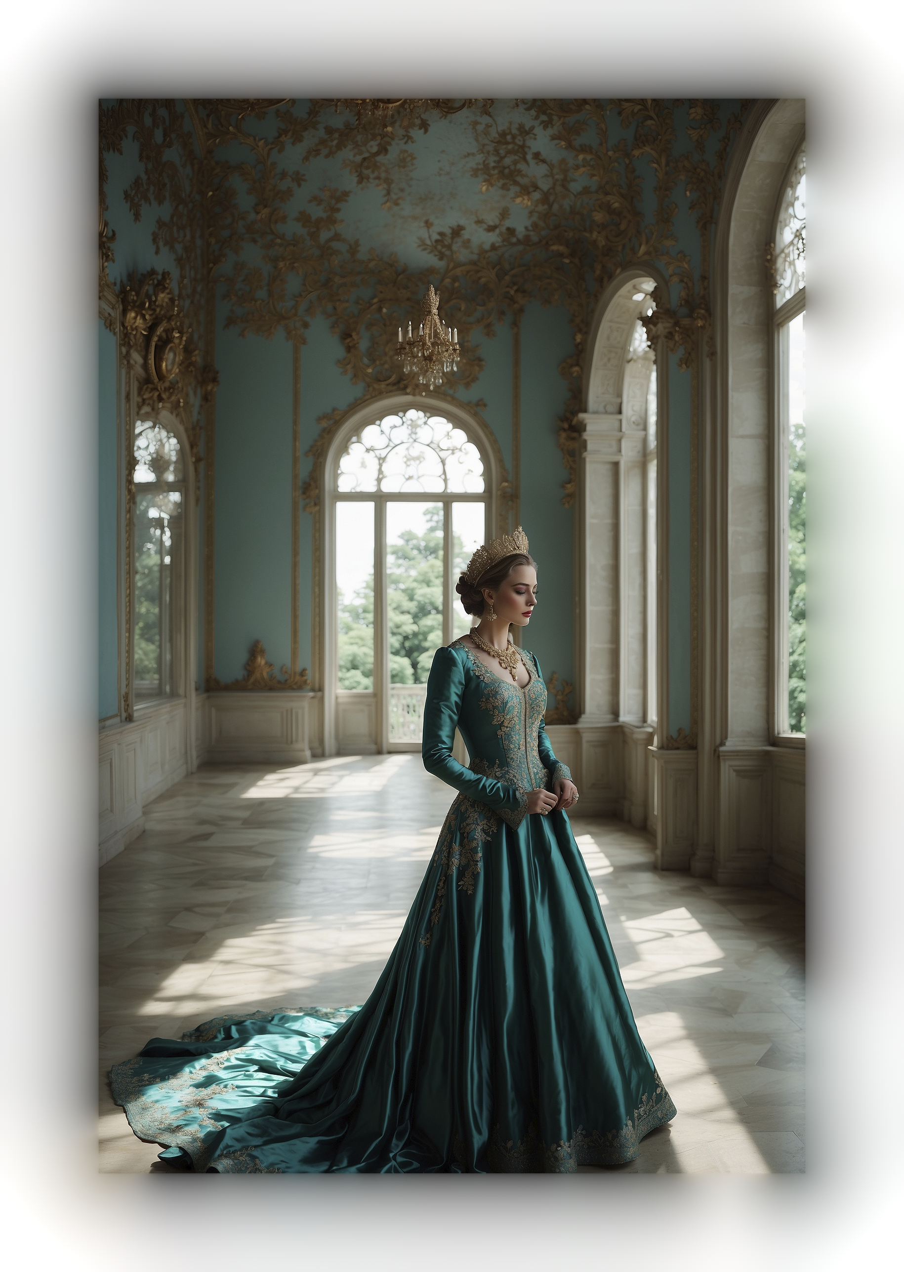
Image generated by AI using Stable Diffusion model through Leonardo AI .
It turned out that merely changing the sign of the diffusion partial derivative equation update could actually sharpen the image. I had worked on blind deconvolution for years when I started working on a diffusion model, and never managed to make even the state-of-the-art method work outside of the nice poster cases (low ISO, low saturation, uniform blur). But this of course needed a regularization parameter to avoid diverging.
This is how the diffuse or sharpen module was born, as a generic framework for all sorts of diffusive or counter-diffusive phenomenon simulation.
Note
In the following, we will use the vocabulary of Fourier harmonic analysis (especially frequency) even though we are not strictly in a such framework, but the wavelets scheme is very close in principle from a signal decomposition into Fourier harmonic series.Continuous model
At heart, the module implements a family of anisotropic diffusion equations of the form
$$ \partial_t u = \nabla \cdot (\mathbf{A} \nabla u), $$
where $u$ is the image and $\mathbf{A}$ is a symmetric positive diffusion tensor that steers the smoothing either along the isophotes, along the gradient, or isotropically.24
The original inspiration in the code is the inpainting model of Qin et al., who couple image structure and texture restoration through anisotropic heat transfer.2 Ansel keeps that spirit, but applies the PDE in a wavelet domain, separately on low-frequency and high-frequency bands, and exposes four user-controlled transport coefficients.
Discrete gradients and anisotropy
For each pixel and each channel, the module extracts a 3x3 neighborhood and evaluates centered first derivatives
$$ \begin{align} g_x &= \frac{u(i+1,j) - u(i-1,j)}{2} \\ g_y &= \frac{u(i,j+1) - u(i,j-1)}{2} \end{align} $$
This is the standard central-difference gradient used in discrete scale-space and diffusion methods.3
The local gradient orientation is then :
$$ \begin{align} \cos\theta = \frac{g_x}{\sqrt{g_x^2 + g_y^2}} \\ \sin\theta = \frac{g_y}{\sqrt{g_x^2 + g_y^2}} \end{align} $$
with the usual fallback to $(1,0)$ when the gradient magnitude vanishes.1 Note that we will avoid computing the expensive $\theta$ angle as the $\arctan2$ function of the $(x, y)$ components, since it will never be used directly in the following.
The anisotropy strength is converted from the user parameter $a$ into a positive coefficient
$$ \alpha = a^2, $$
while the sign of $a$ selects the mode:
- $a = 0$: isotropic diffusion,
- $a > 0$: diffusion aligned with the isophote direction,
- $a < 0$: diffusion aligned with the gradient direction.1
The damping term is then
$$ c^2 = \exp(-\alpha \lVert \nabla u \rVert), $$
which matches the anisotropic diffusion of Qin et al. for inpainting.2
For isophote-aligned diffusion, the tensor written in the local image basis is :
$$ \mathbf{A}_{\perp} = \begin{bmatrix} \cos^2\theta + c^2 \sin^2\theta & (c^2 - 1)\cos\theta\sin\theta \\ (c^2 - 1)\cos\theta\sin\theta & c^2 \cos^2\theta + \sin^2\theta \end{bmatrix}. $$
For gradient-aligned diffusion, Ansel uses the inverted form :
$$ \mathbf{A}_{\parallel} = \begin{bmatrix} c^2 \cos^2\theta + \sin^2\theta & (1 - c^2)\cos\theta\sin\theta \\ (1 - c^2)\cos\theta\sin\theta & \cos^2\theta + c^2 \sin^2\theta \end{bmatrix}. $$
The 3x3 diffusion stencils
Depending on user parameters, we will evaluate for each pixel the $\mathbf{K(A)}$ stencil using one of the $\mathbf{A}$ tensors above.
Given the symmetric tensor $\mathbf{A}$ :
$$ \mathbf{A} = \begin{bmatrix} a_{11} & a_{12} \\ a_{12} & a_{22} \end{bmatrix}, $$
we build the discrete, rotated, anisotropic Laplacian kernel $\nabla \cdot (\mathbf{A}\nabla u)$ as the 3x3 stencil :
$$ \mathbf{K}(\mathbf{A}) = \begin{bmatrix} \frac{a_{12}}{2} & a_{22} & -\frac{a_{12}}{2} \\ a_{11} & -2(a_{11}+a_{22}) & a_{11} \\ -\frac{a_{12}}{2} & a_{22} & \frac{a_{12}}{2} \end{bmatrix}, $$
up to the sign convention mentioned in the source code for the off-diagonal terms.241
In the isotropic case expands to a constant :
$$ \mathbf{K}_{\text{iso}} = \begin{bmatrix} \tfrac14 & \tfrac12 & \tfrac14 \\ \tfrac12 & -3 & \tfrac12 \\ \tfrac14 & \tfrac12 & \tfrac14 \end{bmatrix}, $$
which is the classical Oono-Puri style isotropic Laplacian. Its interest is rotational behavior: compared with the 5-point Laplacian, the angular error is reduced, which matters when diffusion must not privilege the image axes.56 This angular error was evaluated against similar kernels in Rotation-invariant Laplacian for 2D grids .
To understand the effect of direction in diffusion, let’s start with a noisy disc and diffuse it with Ansel :
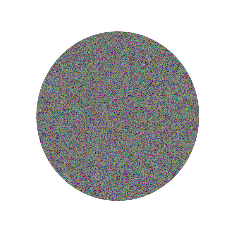

50 iterations of 12 px isotrope diffusion : it’s equivalent to a good old gaussian blur.

50 iterations of 12 px gradient-parallel diffusion : note the feathers (or “sun rays”) close to north/south/east/west positions.
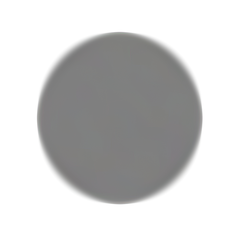
50 iterations of 12 px gradient-perpendicular (isophote) diffusion : it’s an edge-avoiding surface blur, especially close to north/south/east/west positions.
A couple of things are worth mentionning here :
- Only the isotrope blurring yields an achromatic disc, the other retain some large-scaled chroma noise, because the chroma noise creates local gradient variations.
- The anisotrope diffusion is perfect near the north/east/south/west positions of the circle, that is when gradient angle is perfectly aligned on the pixel grid (0° or 90°). In-between, we see discrepancies regarding how direction is dealt with, due to the numerical limitations of a rotated 3×3 square stencil.
The à-trous B-spline pyramid
The multiscale analysis is built from the separable 5-tap cardinal B-spline filter
$$ h_0 = \frac{1}{16}[1,4,6,4,1]. $$
This filter is a compact Gaussian approximation, which is why it appears naturally in spline-based scale-space methods.7 We re-use here the framework introduced by Johannes Hanika for the contrast equalizer module.8
The current implementation uses the historical undecimated a-trous ladder:
The first full-resolution low-pass is
$$ G_0 = h_0 * u, $$
The finest detail band is
$$ H_0 = u - G_0. $$
Coarser levels keep the same image resolution and only enlarge the blur stride by $2^s$:
$$ G_s = h_{2^s} * G_{s-1}, \qquad s > 0. $$
meaning at $s=1$, $h_{2}$ taps are evaluated every next pixel, as $s=2$, $h_4$ taps are evaluated every 4 pixels, and so on…
The band stored at scale $s$ is the difference between two successive low-passes:
$$ H_s = G_{s-1} - G_s, \qquad s > 0. $$
So every band lives on the original image grid (no decimation), and we solve the PDE fine-to-coarse in parallel, by accumulating the solution scale by scale into the output buffer until we add the final residual.1 This scheme avoids stacking up the fine scales correction on top of the coarse scales, as is customary with Gaussian pyramids or multi grid solvers, and has shown empirically better stability in the inverse problem of sharpness reconstruction. This is equivalent to managing the energy of each band separately, in a way that resembles HiFi audio equalizers, but within a 2D spatial framework.
Kernel scale, band scale, and the GUI scale envelope
To study the wavelet scheme properties, we will use the property of the cardinal B-spline of being a Gaussian filter approximation. The Gaussian parameter $\sigma$ controls how blur kernels compose:
$$ G(\sigma_1) * G(\sigma_2) = G\left({\sqrt{\sigma_1^2 + \sigma_2^2}}\right) $$
so Gaussian kernel variances $\sigma^2$ add under convolution.37 By contrast, the variance of a filtered signal $X$ :
$$ \operatorname{Var}[g_\sigma * X], $$
depends on the spectrum of $X$ and is generally not equal to $\sigma^2$. To disambiguate both variances, in the rest of this article, $\sigma$ refers only to the parameter of the Gaussian kernel, never to the square root of signal variance.
To avoid ambiguity, it also helps to separate the low-pass levels from the levels bands:
- $G_0 = h_1 * u$ is the first full-resolution low-pass over the input image $u$,
- $G_s = h_{2^s} * G_{s-1}$ for $s \ge 1$,
- $H_0 = u - G_0$,
- $H_s = G_{s-1} - G_s$ for $s \ge 1$.
So:
- the low-pass index $s$ refers to the blur level $G_s$,
- the band index $s$ refers to the detail band $H_s$ sitting between $G_{s-1}$ and $G_s$,
- every level remains sampled on the original image grid.1
The B-spline filter approximates best the equivalent Gaussian kernel of parameter :
$$ \sigma_B \approx 1.055365. $$
Because Gaussian-kernel variances add under convolution, the effective blur radius of $G_s$ follows directly from the a-trous analysis ladder. Therefore the cumulative low-pass sequence is
$$ G_0; G_1; G_2; G_3; \dots \quad \Longleftrightarrow \quad \sigma_{G_0}; \sigma_{G_1}; \sigma_{G_2}; \sigma_{G_3}; \dots $$
with
$$ \sigma_{G,0} = \sigma_B,\qquad \sigma_{G,1} = \sqrt{5}\sigma_B,\qquad \sigma_{G,2} = \sqrt{21}\sigma_B,\dots $$
and, in general,
$$ \sigma_{G,s}^2 = \sum_{k=0}^{s} \sigma_B^2 4^k = \sigma_B^2 \frac{4^{s+1} - 1}{3}. $$
Equivalently,
$$ \sigma_{G,s} = \sigma_B \sqrt{\frac{4^{s+1} - 1}{3}}, $$
The code uses $\sigma_{G_s}$ to decide how many scales are needed to match the user-requested radius parameter and to weight each band around the user-selected central radius:
$$ w_s = \exp\left( - \frac{(z\sigma_{G,s} - r_c)^2}{r_w^2} \right), $$
where $z$ is the darkroom zoom level (compared to full-resolution raw), $r_c$ is radius_center in the GUI, and $r_w$ is radius.1 By setting those, users define the decay of a sort of discretized “bandwidth” filter centered on an arbitrary frequency. In that sense, $r_w$ is the width of a Gaussian envelope in scale space. It is not the radius of the PDE stencil, nor the radius of a single blur. It is the spread of the gain profile applied to the discrete wavelet bands.
The weighting scheme is stable no matter the zoom level : radii are taken in raw-image (full-resolution) space. When previewing images downscaled in darkroom, the highest frequencies are truncated by the downscaling, so we only apply the wavelets decomposition starting from the highest frequency available and reweigh them according to their equivalent full-resolution radius. This allows a fairly accurate downscaled preview, even though it may hide noisy artifacts appearing at the highest levels.
Bands whose equivalent blur radius $\sigma_{G_s}$ lies close to $r_c / z$ receive the largest gain, while bands farther away are progressively attenuated. A small $r_w$ gives a narrow selection of scales; a large $r_w$ gives a broader and flatter response over neighboring bands.
So the pair (radius_center, radius) should be read as a center and width in scale space. The module does not directly define a Gaussian in Fourier frequency; instead, it defines a Gaussian envelope over the available multiscale bands.1
Generic multiscale PDE update
Let:
- $H_s$ be the stored detail band at band index $s$,
- $G_s$ be the current low-frequency reconstruction used when solving band $H_s$ during synthesis.
At a given band $s$, the code builds four diffusion responses:
$$ \begin{align} D_{1,s} &= p_1 \, K_{1,s}(a_1, G_s) * G_s,\\ D_{2,s} &= p_2 \, K_{2,s}(a_2, H_s) * G_s, \\ D_{3,s} &= p_3 \, K_{3,s}(a_3, G_s) * H_s, \\ D_{4,s} &= p_4 \, K_{4,s}(a_4, H_s) * H_s, \end{align} $$
where:
- $K_{1,s}$ and $K_{2,s}$ are 3x3 anisotropic diffusion stencils applied to the current low-frequency reconstruction $G_s$,
- $K_{3,s}$ and $K_{4,s}$ are the analogous stencils applied to the detail band $H_s$,
- $a_1$ to $a_4$ are 4 user-defined anisotropy damping coefficients (see above),
- $p_1$ to $p_4$ are 4 user-defined PDE update (transport) coefficients (see below),
- the convolution is channel-wise on the sparse a-trous sub-lattice of stride $2^s$.1
All the Laplacian $K$ kernels are applied with the same stride distance as the B-spline blur having been used to produce the wavelet scale $s$ over which they are applied, that is $2^s$. Given that the blur kernel is 5×5 and the Laplacian kernels are 3×3, that means the Laplacian covers a quarter of the blur surface.
All those $K$ are an effort to make the diffuse or sharpen a generic multiscale PDE framework, as they will cross information between $G_s$ and $H_s$ :
| Laplacian evaluated on \ Gradient evaluated on | $G_s$ | $H_s$ |
|---|---|---|
| $G_s$ | $K_{1,s}$ | $K_{2,s}$ |
| $H_s$ | $K_{3,s}$ | $K_{4,s}$ |
The gradients evaluated on $G_s$ are more likely to point toward legitimate image details, and can be used in a sharpening setting to ignore noise. The gradients evaluated on $H_s$ are more sensitive to noise and can be used in a diffusive setting to soften noise. We separate the layer on which we infer image structure (gradient direction) from the layer where we compute the PDE update (Laplacian) and thus the diffusion.
For lack of better term, those $K_i$ responses are linked to GUI parameters called “orders” from first to fourth :
speed, which is the PDE update coefficient,anisotropy, which is the $a$ damping coefficient from the anisotropy tensor above.
We have therefore 4 speed parameters, one for each order :
$$ (p_1, p_2, p_3, p_4) = (\texttt{first}, \texttt{second}, \texttt{third}, \texttt{fourth}), $$
And similarly, 4 anisotropy parameters :
$$
(a_1, a_2, a_3, a_4) = (\texttt{first}, \texttt{second}, \texttt{third}, \texttt{fourth})
$$
The meaning of all that can be translated in layman’s term like so :
- we diffuse structure in the direction of structure ($D_1$, first order),
- we diffuse structure in the direction of texture ($D_2$, second order),
- we diffuse texture in the direction of structure ($D_3$, third order),
- we diffuse texture in the direction of texture ($D_4$, fourth order).
Any $p$ coefficient set to 0 cancels diffusion, any $a$ coefficient set to 0 cancels anisotropy.
The PDE update at scale $s$ is therefore :
$$ U_s = G_s + H_s + \frac{\kappa \, w_s}{\nu_s} \sum_{i=1}^{4} D_{i,s}, $$
where :
- $\kappa$ is the discretization factor, that is $\frac14$ for finite centered differences,
- $\nu_s$ is the regularization parameter that we will see next section,
- $w_s$ is the scale weighting defined at the previous section.
And the final resynthesis is simply :
$$ u’ = \sum_{s=0}^{n} U_s $$
So, if we summarize the whole algorithm, given $u$ the initial image, $u’$ the final one, $n$ the final number of scales :
$$ \begin{align*} s &\in [0, n] \\ G_{-1} &= u \\ G_s &= h_{2^s} * G_{s-1}, \\ H_s &= G_{s-1} - G_s, s\in[0,n] \\ w_s &= \exp\left( - \frac{(z\sigma_{G,s} - r_c)^2}{r_w^2} \right) \\ D_{1,s} &= p_1 \, K_{1,s}(a_1, G_s) * G_s \\ D_{2,s} &= p_2 \, K_{2,s}(a_2, H_s) * G_s \\ D_{3,s} &= p_3 \, K_{3,s}(a_3, G_s) * H_s \\ D_{4,s} &= p_4 \, K_{4,s}(a_4, H_s) * H_s \\ u’ &= \sum_{s=0}^{n} \left[ G_s + H_s + \frac14 \frac{w_s}{\nu_s} \sum_{i=1}^{4} D_{i,s}\right] \end{align*} $$
Some notes:
- $n$ is not an user parameter but is determined with regard to the target final $\sigma$ requested by user radius parameters. This adjusts to zoom level as a byproduct.
- The Gaussian blur is itself the 2D isotrope solution to the heat equation : it is already diffusion.
- Increasing the blur radius is equivalent to letting the diffusion run for a longer time : the signal spreads farther.
- For $s > 0$, $H_s$ actually becomes a difference of Gaussians. At some scaling correction coefficient, the difference of Gaussians is an approximation of the Laplacian of a Gaussian, which itself is an estimation of the Laplacian at a scaling coefficient $\sigma$.
- Applying a (possibly anisotrope) Laplacian over $H_s$ again is equivalent to a 4-th order partial derivative (bi-Laplacian).
Structure of the correction factor
The term that controls the PDE transport is
$$ \frac{\kappa \, w_s}{\nu_s}, $$
In this section, we will define the $\nu_s$ factor.
Defining well-behaved frequency filters for photographs
Photographs are digital reproductions of a latent image throuh an exposure apparatus (diaphragm aperture, sensor ISO sensitivity, shutterspeed) and a discretization (or spatial sampling) apparatus (color filter array, pixel grid). Those are artifacts of the technology used to capture the latent image and do not concern the actual image.
Unfortunately, the capture heuristics regarding exposure and sampling affect how we process the digital image. I have shown on discs at the 3×3 diffusion stencils section, how diagonal edges behave differently from grid-aligned edges (vertical/horizontal), even though I chose the most rotationally-invariant kernels : image content rotation (compared to pixel grid) will change how discrete gradients are evaluated. The concrete implication here is : rotating the image before or after diffuse or sharpen will not yield the same outcome.
But it doesn’t stop there : exposure changes the signal variance too. Given a white signal $X$, its local variance $V_1$ over a sampling window $\mathcal{N}$ is expressed :
$$ \begin{align} V_{1, \mathcal{N}} &= \frac{1}{|\mathcal{N}|} \sum_{i\in\mathcal{N}} (\bar{X} - X_i)^2 \\ & = \frac{1}{|\mathcal{N}|} \sum_{i\in\mathcal{N}} \left(\left(\sum_{i\in\mathcal{N}} X_i \right) - X_i\right)^2 \end{align} $$
If, instead of capturing $X$, we over-exposed the same image by a factor $l$, then the variance of $lX$ would become $V_2$:
$$ \begin{align} V_{2, \mathcal{N}} &= \frac{1}{|\mathcal{N}|} \sum_{i\in\mathcal{N}} (l\bar{X} - lX_i)^2 \\ & = \frac{l^2}{|\mathcal{N}|} \sum_{i\in\mathcal{N}} (\bar{X} - X_i)^2 \\ & = l^2 \, V_{1, \mathcal{N}} \end{align} $$
So the variance of the signal increases with the square of the exposure factor. This matters to us here for two reasons, that can be summarized right now by this : all we do here is changing the scale-wise variance of the image.
First, our B-spline blurring step is a local weighted average, and $H_s$ evaluated at the pixel of coordinates $(x, y)$ can actually be written :
$$ \begin{align} H_s(x, y) &= X(x, y) - G_s(x,y)\\ &= X(x, y) - h_s * X(x,y)\\ &= -\left(\frac{1}{16^2} \sum_{i = -2}^{+2} \sum_{j = -2}^{+2} h_{i + 2} \, h_{j + 2} \, X(x + i, y + j) \right) + X(x, y) \end{align} $$
with $h_{i, j}$ the coefficients of the 5-taps, 2D, B-spline kernel, and $X$ the blurred signal of the previous scale (or the initial image for the first step). We can similarly show that $H_s$ is linearly dependent to the exposure factor. The above equation shows how $H_s$ can be seen as a modulation around a local average : the magnitude of that modulation is not independent from the magnitude of the signal. It means that any smoothing of $H_s$ (carried out as a diffusive process) will have a different weight and a different impact on details whether the image is over-exposed or under-exposed, even though the content is the same.
Said otherwise, smoothing (or conversly, sharpening) then underexposing, or underexposing then smoothing will not have the same effect on details, even though the final overall magnitude (average) of the signal will be the same. This is not what we expect from a well-behaved image filter : the data-representation of the content should not affect how we process the content itself. In the diffusive setting, it is not that damaging, but in the sharpening setting, details in shadows get really oversharpened compared to details in highlights, without any kind of normalization.
Second, the B-spline blur (or its Gaussian best approximation) will change the variance of the signal too. If we express the discrete signal $X$ as a local modulation around the global average $\mu$, we get $X_n = \mu + \epsilon_n$. Then, the B-spline blur applied to $X$ becomes :
$$ \begin{align} G_{0}[n] &= \sum_{k} h_{k} (\mu + \epsilon_{n-k}) \\ &= \sum_{k} h_{k} \, \mu + \sum_{k} h_{k} \, \epsilon_{n-k} \\ &= \mu \sum_{k} h_{k} + \sum_{k} h_{k} \, \epsilon_{n-k} \end{align} $$
Because the coefficients of the $h_{k}$ kernel are normalized and $\mu$ is, by definition, constant over the window of length $k$, we get $\mu \sum_{k} h_{k} = \mu$, meaning that the blur doesn’t change the average value. The variance is then expressed :
$$ \begin{align} \operatorname{Var}(G_0) &= \frac{1}{\mathcal{N}} \sum_{n \in \mathcal{N}} \left(\mu - \left(\mu + \sum_{k} h_{k} \, \epsilon_{n-k}\right) \right)^2 \\ &= \frac{1}{\mathcal{N}} \sum_{n \in \mathcal{N}} \left(\sum_{k} h_{k} \, \epsilon_{n-k} \right)^2 \\ &= \operatorname{Var}\left(\sum_{k} h_{k} \, \epsilon_{n-k}\right) \end{align} $$
From there, we can show that, for white, uncorrelated signals, $\operatorname{Var}(G_0) = \operatorname{Var}(X) \sum_k h_k^2$, and more generally :
$$ \operatorname{Var}(G_s) = \operatorname{Var}(G_{s-1}) \sum_k h_k^2 $$
where $\sum_k h_k^2 = (35 / 128)^2$ for the 5-taps cardinal B-spline 2D filter.
And here again, we have a problem : the same object sampled at some resolution, or at 4 times that resolution, would appear at the same “frequency” one step of wavelets decomposition later, which would make its surface variance $(35 / 128)^2$ lower. But this is purely a sampling artifact. The variance of the object itself can be conceptualized, outside of the image, in a continuous setting, as the local color modulations around its average surface color. While this idealized variance cannot be recovered by any imaging apparatus, the way we handle the signal should at least be stable in variance so we can posit image variance represents the object idealized variance to some constant scaling factor.
This might seem like philosophical concerns until we hit a practical problem of any imaging software : what happens when we preview the effect zoomed in/out ? How do we scale the effect so the downscaled preview is still faithful to the full-resolution result ?
So, all these sampling discrepancies need to be normalized to achieve an image filter that tries to manipulate content regardless of its data representation.
Defining a regularization metric
We have seen above how the signal variance is a relevant metric for what we are doing here : we can trace it through the blurring steps, link it to signal magnitude, and it represents the signal modulation around the average value.
Unfortunately, we don’t have access to a metric of variance once we enter the wavelets decomposition scheme. However, we have seen above that $H_s$ was pretty close, conceptually, to the $(\bar{X} - X_i)$ term of the variance :
- instead of an arithmetic mean, we use a weighted average using B-spline coefficients,
- instead of a global average, we use a local one,
- the B-spline radial nature makes it more rotationally-invariant than any square patch-wise average.
So we will use the $H_s$ band energy, evaluated at the same pixel coordinates as the Laplacian stencil, defined as :
$$ Q_s = \sum_{q \in \mathcal{N}_{3\times 3}} H_s(q)^2. $$
For a slowly-varying, white, uncorrelated signal, $\overline{Q_s} = Q_s / |\mathcal{N}_{3\times 3}|$ becomes close to the scale-wise and patch-wise variance.
The regularization is meant for the sharpening problem, which is ill-defined : in this setting, we increase the energy of each layer $H_s$ and we need a parameter to dock it at bay at some point. This is a common procedure in inverse problems such as denoising and deblurring, for which Total Variation has been used as a regularization scheme for quite some time.
The regularization model we will use is :
$$ \nu_s = \tau + \lambda \, \dfrac{1}{9} \sum_{q \in \mathcal{N}_{3\times 3}} \left(\frac{H_s(q)}{L_s(q)} \right)^2. $$
with the user parameters :
$$ \lambda = 10^{\texttt{regularization}} - 1, \qquad \tau = 10^{\texttt{variance_threshold}}. $$
We have shown above how the signal variance varies with the square of the exposure scaling, and how $H_s$ varies linearly with the exposure scaling. $G_s$ carries the same linear dependency through its property of being a local weighted average.
So, the ratio $H_s / G_s$ is exposure-invariant. By identification, $L_s(q) = G_s(q)$ in the regularization equation, so we use the exposure-invariant band energy :
$$ Q_s’ = \sum_{q \in \mathcal{N}_{3\times 3}} \left(\frac{H_s(q)}{G_s(q)} \right)^2 $$
and its local average :
$$ \overline{Q_s’} = \frac{1}{9} \sum_{q \in \mathcal{N}_{3\times 3}} \left(\frac{H_s(q)}{G_s(q)} \right)^2 $$
Normalizing scale and spatial coverage
The 3×3 Laplacian stencil expands by a $2^s$ stride for each scale $s$, just like the B-spline kernel does : this is the basis of the “à-trous” scheme. The physical space covered by that kernel increases with wavelets scales.
We can show that a 2D Gaussian filter of parameter $\sigma$ changes the original signal variance like :
$$ \operatorname{Var}(g_\sigma * X) = \dfrac{\operatorname{Var}(X)}{4 \pi \sigma^2} $$
Given that $4 \pi \sigma^2$ is the effective disc area covered by the Gaussian filter, this matches a very simple intuition : the Gaussian filter spreads the original modulation (expressed as variance) over a larger surface. That’s diffusion in a nutshell. We derive from that :
$$ \operatorname{Var}(X) \propto \sigma^2 \operatorname{Var}(g_\sigma * X) $$
Between 2 Gaussian blur steps, the variance parameter of the equivalent Gaussian filter varies by :
$$ \begin{align} \Delta \sigma_s^2 &= \sigma_s^2 - \sigma_{s-1}^2 \\ &= \sigma_B^2 \, 4^s \end{align} $$
And from one scale to the other, this radius grows by $\Delta \sigma = \sigma_B 2^s \approx 2^s$, recalling that $\sigma_B \approx 1.05\dots$.
So the evaluation of the Laplacian spatially expands at the same rate (same stride at each scale) as the B-spline or Gaussian filters : the Laplacian implicitly follows the variance spreading across scales, and no additional scale normalization is needed here.
The initial implementation of diffuse or sharpen had a $\sigma^2_s$ boost applied to the $\lambda$ regularization parameter : in practice, that prevents coarse scales from having any visible impact, and limit them to being the support for high-frequency work.
Another attempt was made to normalize $\lambda$ accounting for the fact that $Q_s$ has a decreasing band energy as $s$ increases, so a scale-invariant energy metric led to :
$$ E_s = \frac{4}{(\Delta\sigma_s^2)^2}Q_s $$
Even combined with the $\sigma^2_s$ factor above, that yielded far too much weight on the coarse scales, making it difficult to sharpen at high frequencies while the low ones were already overshooting badly (giving a smudgy look). Both these attempts have been abandonned.
Result
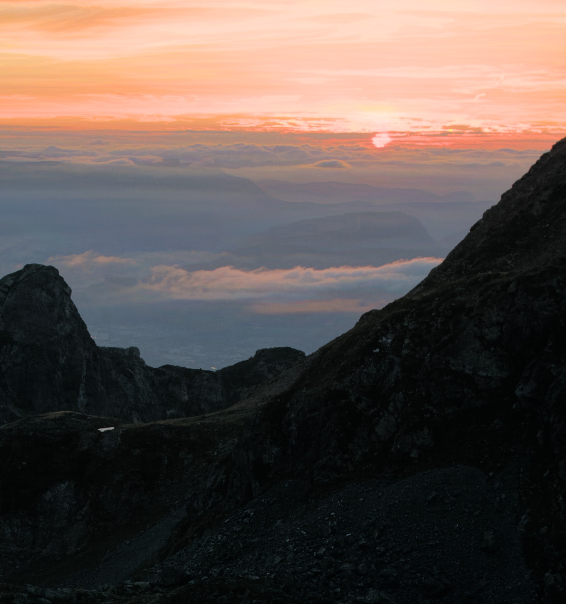

The picture above will look overcooked to most but it’s beyond the point : I have had my share of broken sharpening operators that worked well enough as long as you didn’t push the strength above 2%. Such image filters have zero interest. You learn about algorithms much more by looking at how they fail than at how they succeed in their sweet spot.
This image is the ultimate trap for every sharpening algorithms :
- the foreground is closer and less hazy than the background, so it’s begging to be oversharpened,
- the close foreground is also much darker, so again, easy to push sharpness up the sky there,
- we have a very contrasted mountain ridge begging to produce halos around edges,
- the sun disc in a cloudy sky will be sharpened by most algorithms with dark edges,
- the amount of dehazing required would make the noise explode (this was taken in 2017 with a Nikon D90 at 200 ISO, we are far from current sensors).
So, here we perform a joint denoising & deblurring at large radii. The deblurring uses isotropic counter-diffusion (which best describes atmospheric hazing), on high-frequency and low frequency alike. The denoising uses isophote diffusion on high-frequency, following the gradient sampled in high-frequency. All that was done with no masking, in a single diffuse or sharpen instance.
Overall, we see no edge overshooting and no halos. The dark foreground was mostly ignored, as it should, but we got the details down in the valley back. We got no color shift or chromatic aberrations. I won’t claim this picture is artifact-free, because, when looking up close, we get color streaks and new details that might be actual reconstruction or plain hallucinations of the diffusive model. But the point remain that these artificats, if any, look organic enough to go unnoticed if we don’t have the original image.
This validates the relevance of the multi-scale diffusive scheme, along with the regularization strategy.
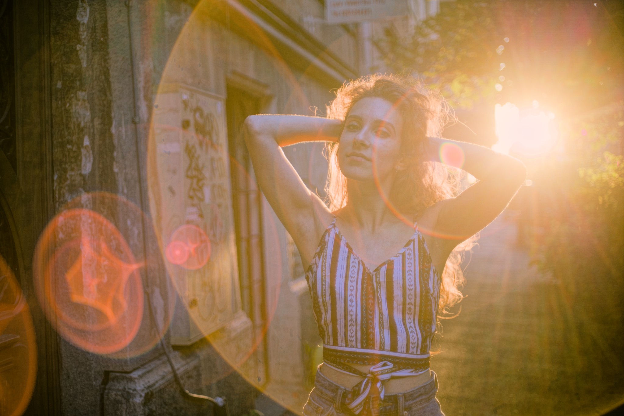
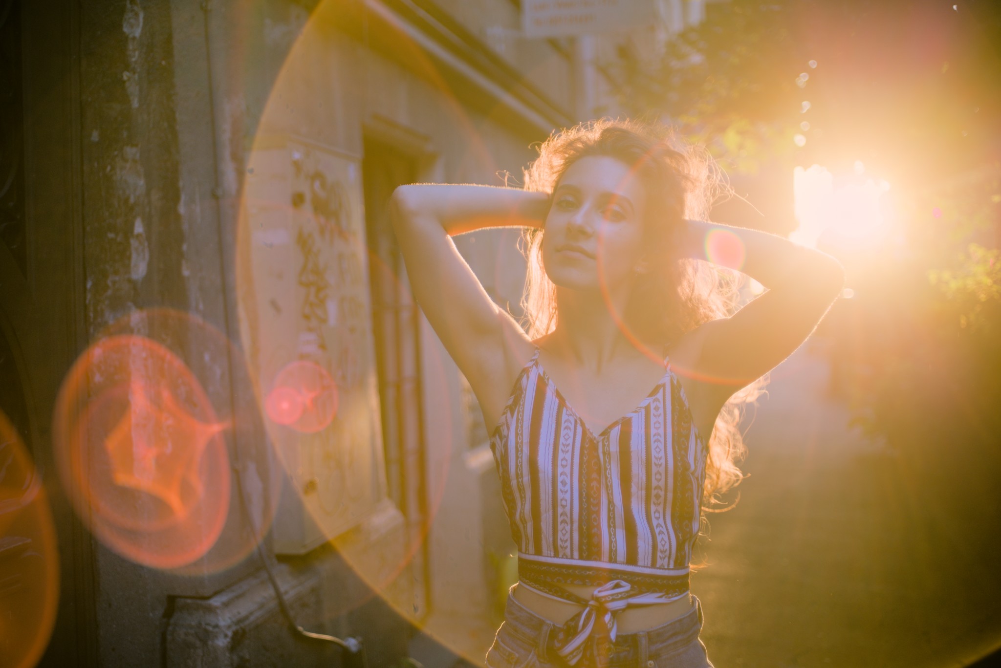
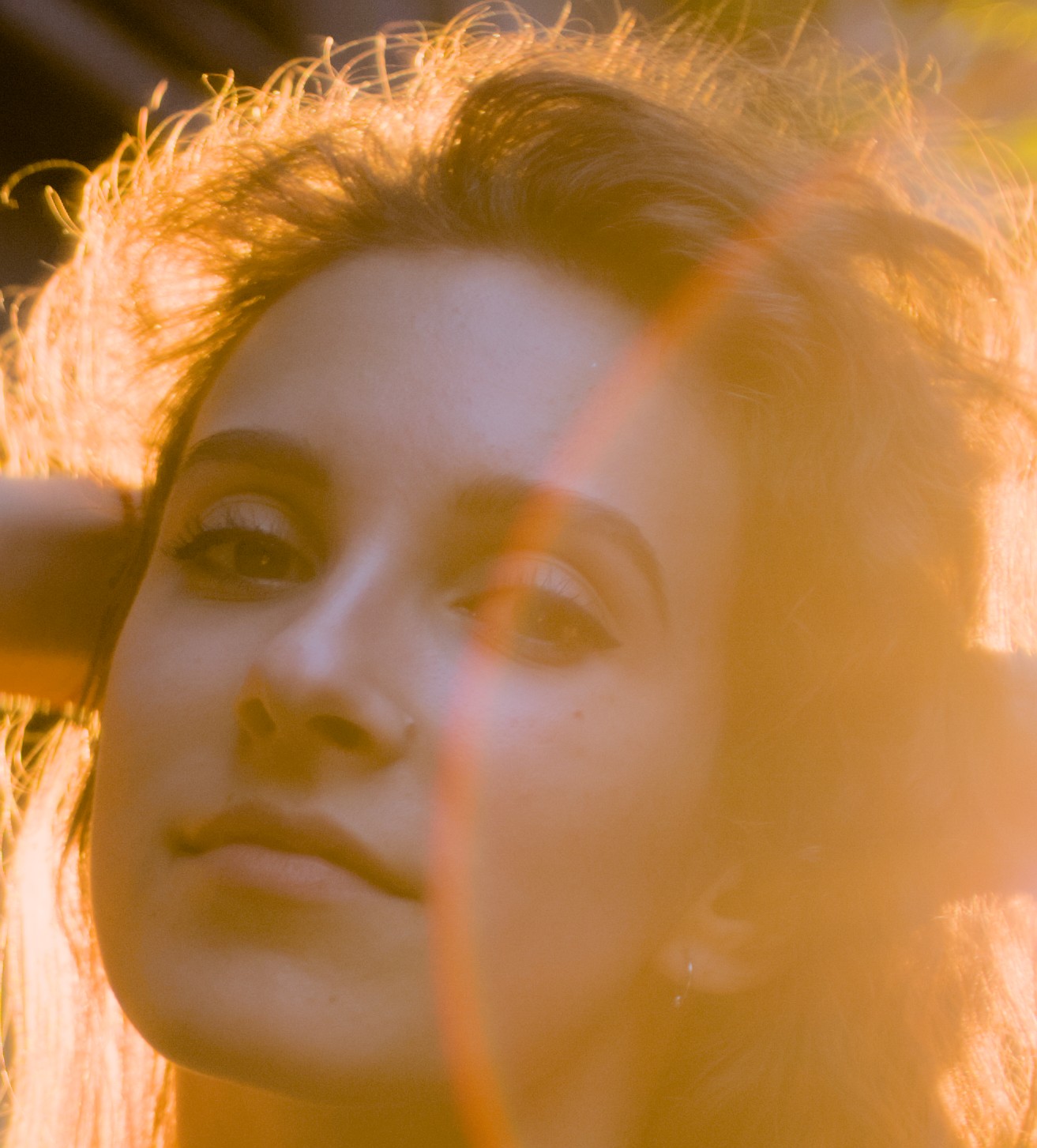
This one was taken with a Sony Alpha 7R Mk 2 but a Konika Hexanon 40 mm f/1.8. This is a pancake lens from the 1970’s, and so the picture is 45 Mpx of beautiful blur. Portraits are less forgiving than landscapes because skin needs to stay healthy when bringing back sharpness. Here we also have all the lensflare and the sun rays that can quickly degenerate.
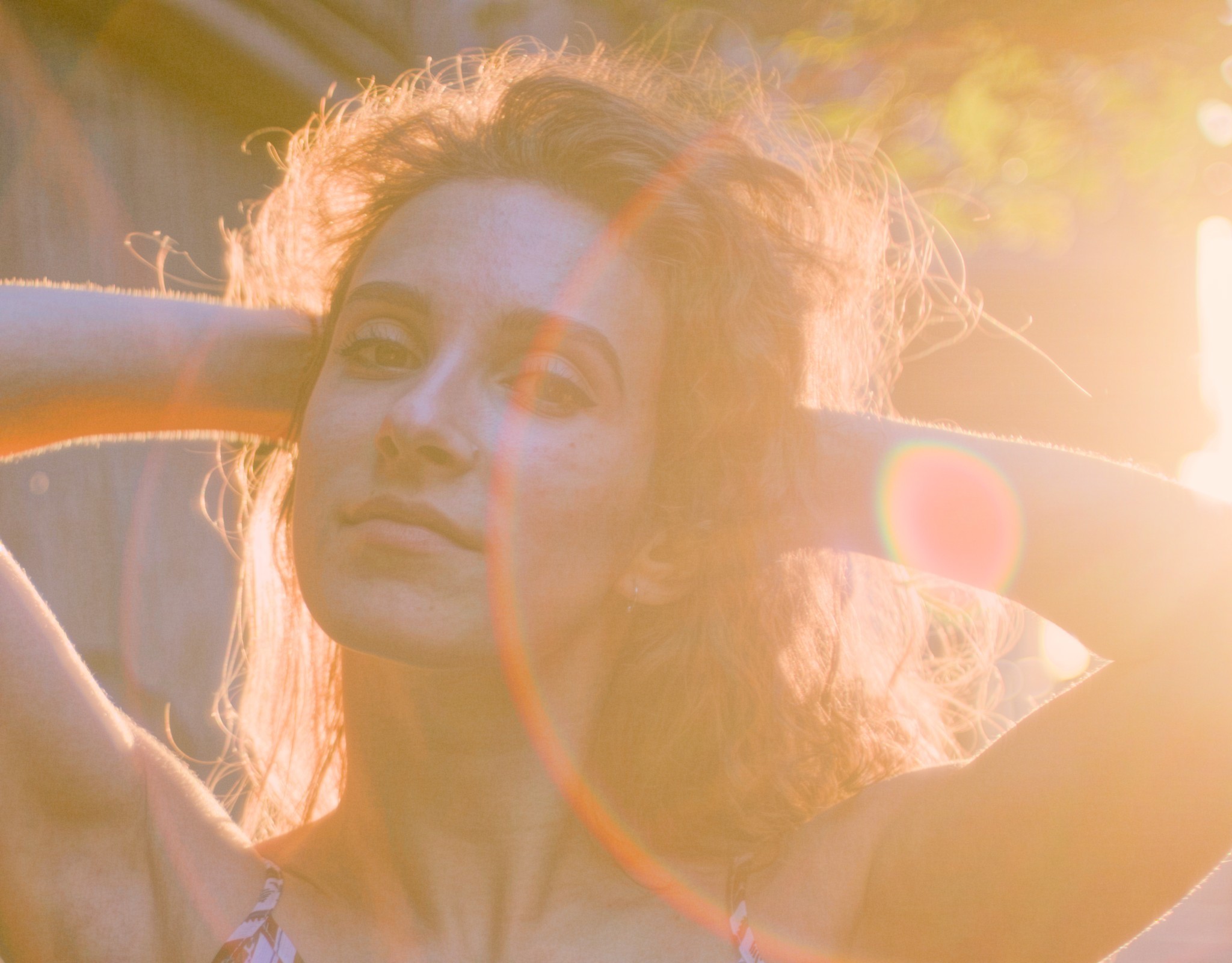
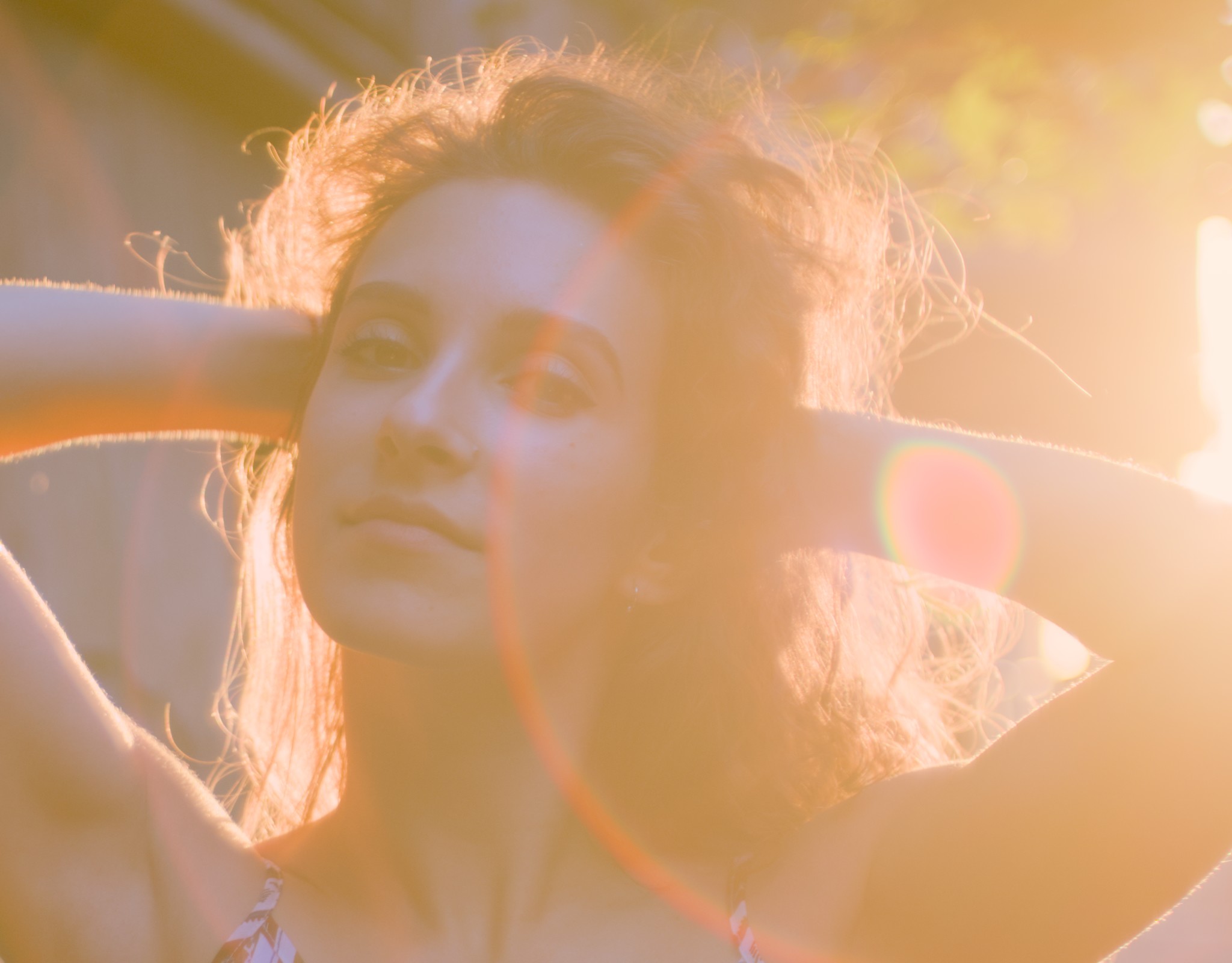
The detail is especially impressive here because we get back the eyebrowes and eyelashes without oversharpening the backlit hair. Overall, there is no ringing, fringing or haloing. Unfortunately, the skin quality has degraded and it’s as far as we can go without masking skin to exclude it. From there, it’s only about bringing back global contrast selectively with a tone curve :

What is specific to Ansel
The scientific references explain the building blocks:
- anisotropic diffusion and heat-transfer inpainting,2
- scale-space and discrete diffusion,34
- isotropic 9-point Laplacians,56
- B-spline Gaussian approximation.7
What is specific to Ansel is the way they are assembled:
- a full-resolution a-trous B-spline pyramid,
- four independently parameterized diffusion operators, split between low and high frequencies,
- an HF band-energy regularizer additionally normalized by the local LF energy,
- zoom-aware scale selection in darkroom preview,
- identical CPU and OpenCL mathematics.1
So the module should be understood as an engineering synthesis of several numerical ideas, not as a literal implementation of a single paper.
Perspectives
The multiscale wavelets scheme of anisotropic diffusion PDE with regularization produces usable photographic results, beyond the mere proof of concept. It allows to leverage joint sharpening and denoising, along with regular oriented diffusion. It also allows to rejuvenate, through software, old lenses that were deemed unfit for high-definition digital photography. The module itself provides a generic PDE playground that can be used in many different ways.
The problem though is that the nature of the settings is grounded into (at least) bachelor-level mathematics and is cryptic to most photographers. Explaining the effect of the parameters is difficult without diving into what they mean mathematically. Trying to rename them by their function instead of their nature is doomed to fail because their function depends on how they are combined together, and whether they are used in the positive or negative value range.
The diffusion setup is pretty straightforward and doesn’t require regularization. It doesn’t need the 4 orders altogether, but only the first and third order settings are enough. In the isotropic setting, it is fully equivalent to a Gaussian blur, which will be less expensive to compute (because non-iterative).
The sharpening setup, along with joint denoising, is more complicated. The only way to make it more user-friendly is to train it as a machine-learning algorithm :
- shoot pairs of clean and blurry/noisy/hazy pictures of the same scene (motion blur, lens defocus blur, soft lenses),
- perform a brute-force parameters sweep of diffuse or sharpen module performing reconstruction of the dirty images, and record the $L_2$ norm of the error between the clean reference images and the attempted reconstructions,
- manually classify the images in binary categories (blurry, noisy, hazy) or by intensity (noise can be measured as PSNR, RMS, … ; radius will probably need to be there too),
- the machine-learning problem becomes : in the 14D space of diffuse or sharpen input parameters, what are the 4 main directions (associated with denoising, deblurring, dehazing, radius) that minimize the error $E = ||\text{clean} - \text{reconstructed}||_2$ ? We are looking for the eigenvectors of those main directions.
- solve that by weighted PLS (partial least-squares) : $Y = X’ B + c$ for $n$ pairs of clean/reconstructed images, where :
- $Y$ is the $4 × n$ vector of categories for each sample,
- $X’$ is the $14 × n$ standardized vector (standardized component-wise : $X_j’ = \frac{X_r - \mu}{\sigma}$) of diffuse or sharpen parameters,
- $B$ is the $14 × 4$ matrix mapping our 14 cryptic D or S parameters to 4 user-friendly parameters (it’s the unknown here),
- $c$ is the residual (scalar or vector depending what fits),
- the $L_2$ norm of the error is used as the PLS weighting (probably injected into an exponential),
- once the matrix $B$ is known (mapping 14D -> 4D), invert it to get the 4D -> 14 D model,
- add an alternative GUI mode exposing the 4 user-friendly parameters, and a GUI <-> parameters layer converting those 4 to the 14 input arguments of D or S (meaning : write the matrix product).
Any other attempt at “simplifying” diffuse or sharpen will only be a silly relabelling job obfuscating the real meaning of the parameters and preventing anybody with the proper mathematical background from understanding it. It would be a shame to make sure that the only few people able to understand it would actually be deterred of even trying. Right now, D or S is difficult to understand, but at least it can be explained. Relabelling controls will not make it easier to understand, but will only add an extra layer of semantic translation between math and GUI, most likely inaccurate and misleading anyway, which will only make it more cognitively demanding to explain and to grasp.
Translated from English by : Automatically generated. In case of conflict, inconsistency or error, the English version shall prevail.
Current implementation in the Ansel source tree:
src/iop/diffuse.c,src/common/bspline.h,data/kernels/diffuse.cl,data/kernels/bspline.cl. ↩︎ ↩︎ ↩︎ ↩︎ ↩︎ ↩︎ ↩︎ ↩︎ ↩︎ ↩︎ ↩︎Chuan Qin, Shuozhong Wang, and Xinpeng Zhang, “Simultaneous inpainting for image structure and texture using anisotropic heat transfer model,” Multimedia Tools and Applications, 56(3), 469-483, 2012. DOI: 10.1007/s11042-010-0601-4 . Metadata: DBLP . ↩︎ ↩︎ ↩︎ ↩︎ ↩︎ ↩︎
Andrew P. Witkin, “Scale-Space Filtering,” Proceedings of the 8th International Joint Conference on Artificial Intelligence (IJCAI), 1983, pp. 1019-1022. Open PDF: IJCAI proceedings . Metadata: DBLP . ↩︎ ↩︎ ↩︎ ↩︎
Andrew P. Witkin and Michael Kass, “Reaction-Diffusion Textures,” Proceedings of SIGGRAPH 1991, pp. 299-308. Canonical DOI: 10.1145/122718.122750 . Open-access copy: Carnegie Mellon Robotics Institute . The implementation comments currently point to a nearby DOI variant. ↩︎ ↩︎ ↩︎
Y. Oono and S. Puri, “Computationally efficient modeling of ordering of quenched phases,” Physical Review Letters, 58(8), 836-839, 1987. DOI: 10.1103/PhysRevLett.58.836 . ↩︎ ↩︎
M. Patra and M. Karttunen, “Stencils with isotropic discretization error for differential operators,” Numerical Methods for Partial Differential Equations, 22(4), 936-953, 2006. DOI: 10.1002/num.20129 . ↩︎ ↩︎
Michael Unser, “Splines: A Perfect Fit for Signal and Image Processing,” IEEE Signal Processing Magazine, 16(6), 22-38, 1999. DOI: 10.1109/79.799930 . Open metadata and reprint links: EPFL . ↩︎ ↩︎ ↩︎
Holger Dammertz, Daniel Sewtz, Johannes Hanika, Hendrik P.A. Lensch, “Edge-Avoiding À-Trous Wavelet Transform for fast Global Illumination Filtering”, Ulm University, Germany, 2010. URL ↩︎
